
Table of Contents
Design Task Functions (DTF)
Design Task Functions are typically higher level functions that will modify data parameters and make repeated use of the various Dose Calculation Functions and Radiotherapy Support Functions to accomplish some type of “optimal” device or plan design.
Aperture Design
Below is a list of the most common aperture design task function and a brief explanation of their intended usage (Specific details of each function, argument parameters, and return values are provided at the Dosimetry App Manifest Guide).
- compute_aperture:
- Compute the aperture without smoothing.
- Recommended mill radius value is is 4.7625mm (0.1875“) and advised to be no less than 2.38125mm (0.09375”) to allow for accurate machining.
- compute_smoothed_aperture:
- Compute an aperture smoothed with a vertex shift on all targets and organs
- Recommended mill radius value is is 4.7625mm (0.1875“) and advised to be no less than 2.38125mm (0.09375”) to allow for accurate machining.
- smooth_aperture:
- Smooth an existing aperture with a vertex shift.
- get_field_rect:
- Gets the bounding box (in BEV) for the aperture opening (at true size not projected).
- compute_aperture_projection:
- Compute the projection of the aperture onto the plane with the given Z depth
- compute_aperture_3d_shape:
- Computes the final physical aperture device as a triangulated mesh
- make_aperture:
- Builds an aperture using the given point list.
- Recommended mill radius value is is 4.7625mm (0.1875“) and advised to be no less than 2.38125mm (0.09375”) to allow for accurate machining.
- remove_polyset_holes:
- A polyset's holes defined an aperture's floating islands. By removing the polyset holes, the resulting computed aperture will contain no islands.
- This function removes the holes from a polyset of an existing aperture (e.g.: Call compute_aperture() and using the polyset from the returned aperture call remove_polyset_holes(). Then replace the original aperture polyset with the polyset returned from remove_polyset_holes())
- apply_mill_radius:
- This function applies a machinability enforcement using a tool mill radius to a polyset of an existing aperture. The resulting polyset shape will not have corners that produce machined under cutting for the mill radius defined.
Geometry
A beam-limiting device is typically referred to as an aperture. It limits the lateral extent of the radiation field, typically such that the beam’s eye view (BEV) projection of the target is circumscribed including provision for a penumbral margin. Since the user specifies the bixel grid parameters, a function must be available to allow for computation of the bounding field for the aperture shape to allow users to compute dose with an acceptable bixel grid.
The aperture device is modeled as one or more open (i.e. the radiation can pass through the defined shape) or closed (i.e. the radiation cannot pass through the defined shape) contours. The actual device blocking is achieved by shaping a high density material, either milled or with a multi-leaf collimator. The contour shapes are modeled at their intended position Zb along the beam axis. The overall aperture is bounded by the mounting apparatus that holds the aperture (typically creating circular or rectangular bounding aperture shapes).
The contour shape can be constrained by the ability to mechanically construct the shape. Milling can be assumed as the primary mode of construction, with a recommended mill radius value is is 4.7625mm (0.1875“) and advised to be no less than 2.38125mm (0.09375”) to allow for accurate machining.
Aperture beam-limiting devices have a physical thickness which is ignored in the beam model. Only the aperture opening shape is considered during any Dosimetry App calculations. Apertures are considered to be infinitely thin and thickness of the devices and slabs will be ignored for divergence and on/off blocking (See Slopsema).
Refer to Beamline Representation for device positioning.
Computing an Aperture Shape
This example will provide a high level walk through of calling the compute_smoothed_aperture function (note compute_aperture is simply a reduced version of this function so this example applies equally to both functions). The code here is meant to be used as a guide on the process to follow and functions/data types to construct. The returned value is the computed geometric shape of the aperture (projected to the given downstream position) based on the arguments passed into the calculation request.
- Construct a beam_geometry
// beam_geometry(std::vector2d sad, matrix<4,4,double image_to_beam);
// sad: The apparent source-to-isocenter distance of the beam. A beam can have different apparent source positions
// in the X and Y directions, so SAD is a two-dimensional value.
beam_geometry geometry(make_vector(main_sad, main_sad),
    rotation_about_axis(make_vector(1.0, 0.0, 0.0), angle<double,degrees>(angle<double,degrees>(180.))) *
    rotation_about_axis(make_vector(0.0, 0.0, 1.0), -angle<double,degrees>(0.)) * translation(-make_vector(0., 0., 0.)));
- Construct a triangle_mesh of the target for the aperture
// struct_geom is a structure_geometry data type representing the desired contoured target volume
triangle_mesh volume = compute_triangle_mesh_from_structure(struct_geom);
- Define aperture_creation_params for aperture geometric properties
aperture_creation_params ap_params;

ap_params.targets.push_back(volume); // Add meshed target to list of targets
ap_params.target_margin = 5.0; // Set margin around targets (5mm)
ap_params.view = compute_beamline_view(geometry, make_vector(0., 0., 0.)); // Set the beam source view(isocenter at 0,0,0)
ap_params.mill_radius = 1.6; // Set the tool radius used during aperture machining (1.6mm)
ap_params.downstream_edge = 100.0; // Set the distance from patient side surface to isocenter along CAX (100mm)
- The aperture_creation_params are then sent to the dosimetry app as calculation requests following thinknode™ calculation request examples.
// Compute the aperture shape. Parameters are: aperture_creation_params, smoothSize, iter, beam_geometry
aperture aper = compute_smoothed_aperture(ap_params, 1., 5, geometry);
Dose/Image Based Aperture Shape
Using exposed Dosimetry App functions an existing dose image can be used as a target structure for aperture creation. The compute_triangle_mesh_from_image function can be used to create a target from a dose iamge at a specified iso-level.
Specific details of each function, argument parameters, and return values are provided at the Dosimetry App Manifest Guide.
// Create a target structure at the 50% isodose line.
triangle_mesh dose_structure = compute_triangle_mesh_from_image(image_50_dose, 50);
// Push the target to the aperture_creation_params
aperture_creation_params ap_params;
ap_params.targets.push_back(dose_structure);
Point vs Dual Source
Point (single) and Dual Source apertures are created in roughly the same manner. When defining a beam_geometry for the aperture, the SAD vector2d automatically defines the source type of the aperture.
Single Source
The SAD IEC-X and IEC-Y values used during construction of the beam_geometry are identical for constructing apertures for Single Point Source machines.
// sad: The apparent source-to-isocenter distance of the beam. A beam can have different apparent source positions
// in the X and Y directions, so SAD is a two-dimensional value, however, for a Single Point Source machine
// these values match.
double main_sad = 1000.0;
beam_geometry geometry(make_vector(main_sad, main_sad),
    rotation_about_axis(make_vector(1.0, 0.0, 0.0), angle<double,degrees>(angle<double,degrees>(180.))) *
    rotation_about_axis(make_vector(0.0, 0.0, 1.0), -angle<double,degrees>(0.)) * translation(-make_vector(0., 0., 0.)));
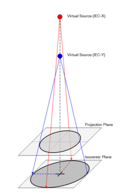
Dual Source
The SAD IEC-X and IEC-Y values used during construction of the beam_geometry are different for constructing apertures for Dual Source machines.
// sad: The apparent source-to-isocenter distance of the beam. A beam can have different apparent source positions
// in the X and Y directions, so SAD is a two-dimensional value, with non-matching values for a Dual Source machine.
double IEC_X = 1050.0;
double IEC_Y = 1000.0;
beam_geometry geometry(make_vector(IEC_X, IEC_Y),
    rotation_about_axis(make_vector(1.0, 0.0, 0.0), angle<double,degrees>(angle<double,degrees>(180.))) *
    rotation_about_axis(make_vector(0.0, 0.0, 1.0), -angle<double,degrees>(0.)) * translation(-make_vector(0., 0., 0.)));
Aperture Mill Radius and Smoothing
Enforcing machinability of the apertures at all evaluation steps is required in order to achieve plan vs. actual. Determining the machinable aperture shape is accomplished by performing an offset of the current “unmachinable” aperture shape by the radius of the final milling tool (in either the inward or outward direction) and then re-offsetting this result by the same distance. Machinability is enforced during aperture computation by using the mill_radius parameter of the aperture_creation_params.
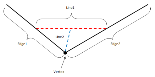
Additionally, smoothing can also be explicitly used to further simplify the aperture shape. As shown in figure 4 below, a line segment (Line1) is created using the center points of the two edges that touch the vertex. A second line segment (Line2) is created going from the vertex to the center point of Line1. The vertex will be shifted along Line2 according the the smoothSize parameter of the compute_smoothed_aperture function. The value of smoothSize should be set between 0.0 and 1.0, indicating how far along Line2 the vertex will shift (0.5 will shift it to the center of Line2, and 1.0 will shift it to the intersection of Line1 and Line2). The iter parameter will indicate how many times the smoothing algorithm will act on the given aperture, with higher values resulting in more smoothing.
The images below provide an exaggerated visual explanation of the creation options for aperture smoothing and mill radius.
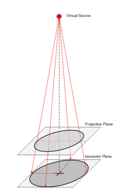
- figure 3: shows the beam setup of the example aperture
- figure 4: shows an example diagram of the smoothing algorithm.
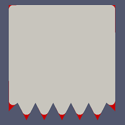
- figure 5: shows a resulting aperture shape with no mill radius and no smoothing applied to the aperture creation parameters
- Note: Recommended mill radius value is is 2.3815mm (0.09375“) and advised to be no less than 0.79375mm (0.03125”) to allow for accurate machining.
- figure 6: shows a resulting aperture shape (black) with a large mill radius applied but not utilizing smoothing options in the compute aperture process.
- figure 7: shows a resulting aperture shape with a large mill radius applied to the aperture creation parameters and smoothing options using the compute_smoothed_aperture function.


Aperture Shape Manipulation
The aperture_creation_params hold the following parameters that can be optionally used with the compute aperture functions to manipulate the resulting computed aperture opening:
- aperture_centerlines
- aperture_half_planes
- aperture_corner_planes
- aperture_organs
- aperture_manual_override
Below is a brief explanation of each of the manipulation tools and their intended effect (Specific details of each argument parameter are provided at the Dosimetry App Manifest Guide).
Example usage:
aperture_creation_params ap_params;
//...
// Set the rest of the aperture_creation_params necessary
//...
ap_params.overrides.push_back(aperture_manual_override(make_polyset(poly), true));
ap_params.half_planes.push_back(aperture_half_plane(make_vector(0., 0.), 45.));
aperture aper = compute_smoothed_aperture(ap_params, 1., 5, geometry);
Structure Centerline
Data struct aperture_centerline
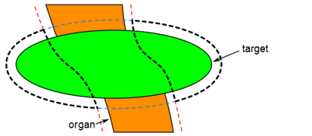
The aperture centerline defines a geometry using the centerline of a structure and a fixed width margin to create a region to remove from the aperture opening. In figure 8 the original aperture shape (blue), structure projection (orange), structure centerline projection (dotted red), and margin (dashed red) are shown. The resulting shape is the combination of the structure_centerline and the original aperture opening shape. The resulting final aperture shape is down in dashed black.
Aperture Organ
Data struct aperture_organ
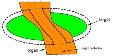
The aperture organ defines a geometry that can be used to clip the aperture opening by the projection of the structure (into BEV), and if applicable, expanded by a margin. By setting the occlude flag, the projected organ shape used for clipping can be limited by the targets if the target is between the source and the organ.
In figure 9 the original aperture shape (blue) and organ structure (red) are shown. With occlude organ by target set to false, the organ outline is projected to the aperture plane to limit the aperture opening shape. By setting the occlude organ by target to true, the target limits the organ projection to the aperture downstream edge plane, thus the organ projection has no effect on the aperture opening shape. The resulting final aperture shape is down in dashed black.
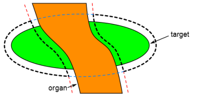
In figure 10 the original aperture shape (blue) and organ structure (red) are shown. Because the organ is in front of the target (in BEV) the organ shape will always be projected to the aperture downstream edge plan and limit the aperture opening. The resulting final aperture shape is down in dashed black.
Manual Override
Data struct aperture_manual_override.
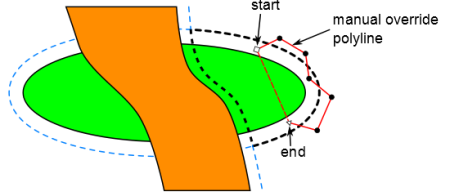
Manual override allows the manipulation of the aperture opening using a constructed polyset shape. Coordinates of the points making up the polygon at to be specified in BEV at the plane of the aperture downstream edge. The aperture opening can either be expanded to or limited based on the specified shape of the override polygons. figure 11 shows the aperture opening (black) and the override polygon (red). The override polygon can expand or limit the shape of the aperture opening based on the flags passed into the aperture_creation_param.
Aperture Half & Corner Planes
Data struct aperture_half_plane and aperture_corner_plane
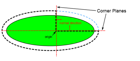
The aperture half and corner planes define a geometry that can be used to remove the portion of the aperture opening in the region on the positive sides (side to which the normal points) of the planes. This feature is necessary in order to create match field aperture devices. In figure 12, the first plane is defined by the origin (0., 0.) and a normal direction of 0 degrees (along the positive x axis). The second plane is defined by the same point, and a normal direction of 90 degrees (along the positive y axis). The result (black) shows how the aperture opening is clipped by removing from the shape anything that is on the positive side of both planes. This same principle can be used with the aperture_half_plane parameter, but instead only specifying one plane to clip the aperture by.
Range Compensator Design
The following example assumes you are familiar with the dosimetry functions and types. These examples will provide a rough process of creating a proton range compensator surface in C++ using pre-existing libraries. The code here is meant to be used as a guide on the process to follow and functions/data types to construct.
- compute_optimized_rc:
- Compute the optimal range compensator for an SOBP field with or without an existing dose.
Refer to Beamline Representation for device positioning.
Range Compensator Optimizer Options
The rc_opt_properties data type stores the optimizer properties needed for a range compensator optimization. Here target requirements, smearing, shifts, current and patch dose can be set.
The interation_count parameter of the rc_opt_properties struct is used to set whether to create a “ray tracing” (i.e. geometric) range compensator or a dose based optimized range compensator. Note that using iteration counts performs a dose calculation per iteration, so it may take considerably longer.
// The maximum number of iterations for the optimization to run.
// Setting iteration_count = 0 creates a geometric only non optimized range compensator.
int iteration_count;
Compute an Optimized Range Compensator
This example will provide a high level walk through of calling the compute_optimized_rc function. The code here is meant to be used as a guide on the process to follow and functions/data types to construct. The returned value is the computed proton_degrader based on the arguments passed into the calculation request.
The compute_optimized_rc function takes the following input data types that must be constructed prior to calling the function:
// Compute the optimal range compensator (RC) for an SOBP field with or without an existing dose.
api(fun monitored)
// A nurbs range compensator.
proton_degrader
compute_optimized_rc(
    // Image 3D of patient stopping power values.
    image3 const& stopping_power_image,
    // The properties of the beam for which an RC is to be computed.
    beam_properties const& beam_props,
    // The SOBP calculation layers for the desired range and mod.
    std::vector<sobp_calculation_layer> const& layers,
    // The aperture for this beam.
    aperture const& aper,
    // Material properties to use for the resulting RC.
    proton_material_properties const& rc_material,
    // The downstream position of the RC on the side nearest to the patient.
    double rc_patient_side_edge,
    // Target(s) for range compensator construction.
    std::vector<triangle_mesh> const& targets,
    // Optimization properties to use for range compensator design.
    rc_opt_properties const& rc_opts);
Patch Field Range Compensator
A patch field range compensator can easily be created using the target(s), ct image, and pre-existing dose. The rc_opt_properties data type created prior to range compensator optimization can optionally take in a current_dose which will be used along with the target(s) distal surface to determine the appropriate range compensator surface. In combination with the patch_distal_dose value, the range compensator surface can be optimized to include the current dose the target has already received.
The figure 13 example below shows a brief explanation of the usage:
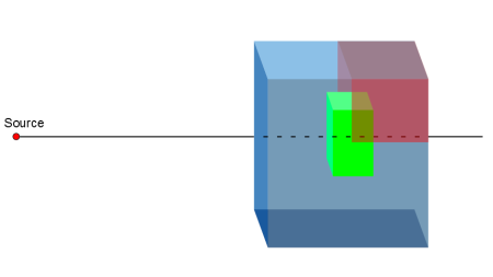 Fig. 13: Range Compensator Patch Field
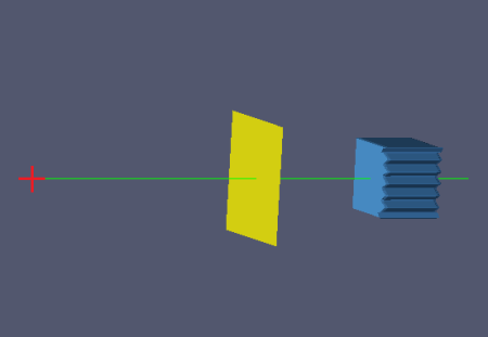
The target (green) is shown within the 3D image (blue & red) that represents the current dose of the target that has been delivered from another field angle. The blue values of the image represent zero dose while the red 100%. Passing this current_dose image and a patch_distal_dose of 20 to the rc_opt_properties will limit the range compensator distal surface to the target distal surface while taking consideration of the 20% isodose line of the current dose.
An approximation of the resulting range compensator surface is shown in figure 14 below.
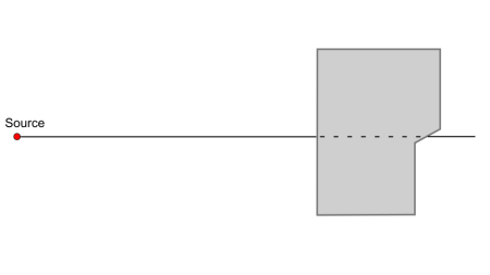 Fig. 14: Resulting Range Compensator w/ Patch Dose
USR-001
.decimal LLC, 121 Central Park Place, Sanford, FL. 32771