
Table of Contents
Dose Calculation Functions
Dose Calculation Functions rely heavily on the Radiotherapy Support Functions and may take as an input the output produced by the Design Task Functions.
Dose Functions
Below is a list of the most common PBS and SOBP dose calculation functions and a brief explanation of their intended usage (specific details of each function, argument parameters, and return values are provided at the Dosimetry App Manifest Guide).
PBS Dose Functions
- compute_pbs_pb_dose:
- Compute the dose for a PBS field to a list of dose points
- compute_pbs_pb_dij:
- Compute the dose for a PBS field to a list of dose points; this version returns a Dij matrix that captures the individual contributions from every physical PBS spot to every dose point
- compute_pbs_pb_dose_to_grid:
- Compute the dose for a PBS field to a regular dose grid; the result is returned as an image covering that grid
SOBP Dose Functions
- compute_sobp_pb_dose:
- Compute the dose for an SOBP field to a list of dose points
- compute_sobp_pb_dij:
- Compute the dose for an SOBP field to a list of dose points; this version returns a Dij matrix that captures the individual contributions from every bixel to every dose point
- compute_sobp_pb_dose_to_grid:
- Compute the dose for an SOBP field to a regular dose grid; the result is returned as an image covering that grid
- compute_sobp_pb_dose_to_adaptive_grid:
- Compute the dose for an SOBP field to a regular dose grid using adaptive grid refinement. The initial dose computation is done at a grid with half the resolution (i.e., 1/8 as many voxels), and the remaining points are calculated selectively based on the dose gradient between their neighbor; the result is returned as an image covering that grid
- compute_sobp_pb_dose_for_bixel:
- Compute the dose for an SOBP field through a single bixel to a list of dose points
- compute_pdd:
- Computes the PDD for the given machine with the provided parameters
The result of each of the dose calculation functions is a scalar dose value at each of the prescribed calculation points (unless otherwise specified). All dose calculation functions require an input “machine model”, and the output unit for each function matches the units used in the machine calibration during the commissioning process (additional details on commissioning a machine model can be found here) . Note there is a direct one-to-one correspondence between the provided dose calculation points and the resulting dose values (i.e. position within the point position and dose value arrays are consistent).
Dose Calculation Modeling
The following general description applies to both PBS and SOBP dose calculations for the Astroid Dosimetry App. Following this general description of the Astroid dose engine, details specific to SOBP calculations will also be provided.
General Dose Calculation Method
Normal use of the dose calculation functions will involve calculation of dose in highly heterogeneous patient geometries. This normal use is usually considered the worst case type of calculation since various size scales and stopping power ranges exist in the computational region, such as small, boney protrusions (head & neck), large bone cross-sections (spine & pelvis), small air cavities (sinus), and large low density regions (lungs). As such, it is important to utilize stable and well trusted computational approaches to dose calculation, such as the Hong model that the Dosimetry App utilizes. The Hong model considers the effects of devices upstream of the patient and the interaction of protons in heterogeneous medium.
In the analytical dose calculation model, we trace the bixel central axis through the voxel grid and compute the radiological depth as a function of position z along the bixel central axis. For each calculation point p=(x,y,z) we compute the diffusion spread σ(z) (per Hong et al.) and compute the dose d to p
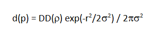 where DD(ρ) is the measured dose of a large-area proton field with energy R.
The analytical model does not “naturally” accommodate the halo protons. These are considered separately as described elsewhere.
The analytical model thus uses the grid only to compute the proton radiological depth ρ at the geometric location (z) of a point (in the bixel (or beam) coordinate system). The analytical model considers the effect of a range-compensator/shifter by reducing the proton range R to R-t and increasing σ by the additional scatter created in the range-compensator/shifter material.
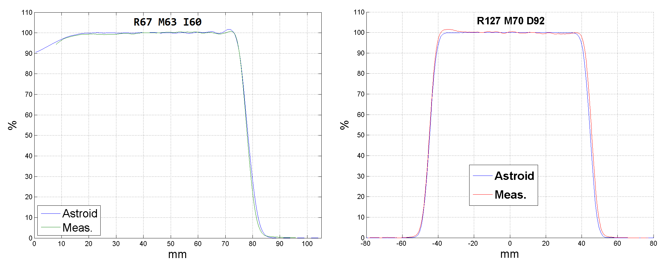
Refer to the Known Application Limitations that details the limitations of the Hong et al calculation method used by the Dosimetry App in respect to heterogeneities and material density. Also, it is expected that the algorithms be utilized only within common clinical range and modulation levels, which at this time include up to about 320mm range and 200mm modulation, and that during commissioning the full range of clinical PBS energies and SOBP range/mod pairings be tested to verified correctness for the user defined machine models. Representative dose results for homogeneous tissue are given below to demonstrate the typical accuracy levels expected for this application.
SOBP Pristine Peak Modeling
An SOBP calculation yields the dose deposited by a spread-out Bragg peak (SOBP) field. An SOBP field is composed of a set of 1 or more pristine peaks that vary in relative intensity to produce a uniform dose over a longitudinal region. The lateral intensity of each pristine peak of an SOBP field is static and either uniform or Gaussian domed. The SOBP pristine peak data is in the form of a sobp_calculation_layer data type in the Dosimetry App.
The beam delivery system (BDS) characterizes SOBP’s in terms of range R and modulation M. This pair is (1) used by the DCF to create (algorithmically) a set of pristine peaks that comprise the SOBP and is (2) used to select the corresponding SOBP on the actual delivery equipment. The use of (R,M) for the latter may require a user or equipment translation to perhaps intermediate parameters.
An SOBP is modeled as the superposition of pristine peaks Ri, with P98 ~< Ri ~< Rs. Each peak Ri is appropriately weighted by Wi such that SOBP = Sum(Wi Ri); see figure 2.
figure 2 shows an SOBP of (R=160 mm, M98=100 mm). This specification reflects the practice where the R of the deepest pristine peak is used to specify the range while the R of the SOBP, itself, is 158.5mm. Note that the M90 (the difference between R90 and the proximal R90) is 129.5 mm. Thus, the SOBP specification is dependent on the institutional practice of calibrating the delivery system and the correspondence with the planning system. The SOBP is constructed from 19 pristine peaks.
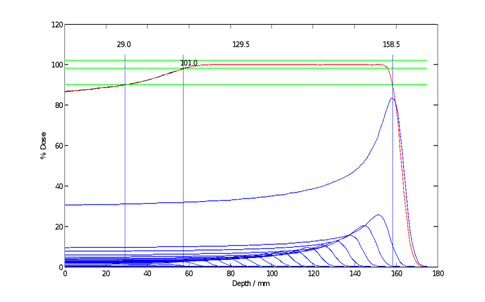 Fig. 2: Representative SOBP Construction
The non-finite source size can cause a “softening” of the SOBP P98 knee when the range-modulation system uses finite thickness shifters that shift in and out of the primary beam. The algorithm models the source explicitly if needed (see Kooy 2008 “XiO SOBP Commissioning”) in a scattering system. The pristine peak Ri is a pristine peak depth dose at infinite SAD (i.e. “TMR” like). The depth-dose is directly or indirectly derived from measurements depending on the scattering system.
SOBP Off-Axis Ratios
The off-axis ratio, OAR, can be (optionally) provided to many of the available SOBP dose calculation functions to allow for improved matching of the results based on the lateral variation of the users actual treatment machine. The OAR is defined as:
 where the profile is measured at a fixed plane at position z along the beam CAX (with z=0 at isocenter and positive z toward the source) and corrected for measurement in the plane at z by projecting back to the isocentric plane and onto a spherical surface with radius SAD. The OAR data is provided on a rectilinear grid using an image data type. The OAR data is used to scale the initial pencil-beam intensity throughout the field.
Dose calculation point distributions
For empirical dose calculations, such as described here, the dose is calculated to a point. The dose to a point is assumed to represent the dose within a spatial extent around that point. Gradients in the dose distributions and variable organ sizes necessitate the distribution of points at sufficient resolution to have the dose at the point accurately represent a volume region (typically a rectilinear dose “voxel”) and to represent dose throughout an organ. The user is free to provide lists of points that are distributed within structures, along structure surfaces, or in any other form. The user is responsible to define the computational resolution commensurate with the clinical assessment.
The dose calculation point coordinates are assumed to be arbitrary with respect to one another. This provides for an independence of accuracy in relation to the number of dose calculation points utilized. In other words, the value of dose computed at a point is independent of the number and distribution of any other points. While the resolution and arrangement of points is important when computing volumetric or other interpolated data, the dose calculation accuracy is such that it is independent at each point. The requestors of the dose calculation service are responsible to specify a list of points commensurate with the desired manipulation of the dose results. It should be noted that dose data is only computed at the provided points, therefore care must be taken to ensure that point distributions cover the entire range of interest for the problem at hand (dose is provided at all points listed even if they are outside the bounds of the patient contour or stopping power image data, as this is a necessary behavior for certain types of calculations).
In order to help users compute dose results that allow for straight-forward computation of volumetric data, the compute_sobp_pb_dose_to_grid2 function is supplied. This function computes dose at a regularly spaced grid of points specified by the user and returns the dose results which represent the dose values at the center of each cell (voxel) within this grid.
In addition to this specific dose calculation function, there are several other helper functions available that can help users quickly generate point lists distributed throughout space. The get_points_on_grid_1d, get_points_on_grid_2d, and get_points_on_grid_3d functions create points distributed along a line, a plane, or a rectangular box region, respectively. Just as when using the compute_sobp_pb_dose_to_grid2 function, the data returned when calling a dose calculation using points generated from one of the above functions should be interpreted as the dose value at the center of the grid cell. Also available is the get_points_on_adaptive_grid function, which creates a point list based on a previously constructed adaptive_grid (see the adaptive_grid data type in the Manifest for more information about how to interpret these results).
An additional concern when utilizing the dose calculation functions is the specification of patient tissue data. This information is provided to the dose calculation using an image3 where each pixel value corresponds to the average stopping power value over the pixel volume (can be thought of again as cell-centered data values). Typically this data is generated by converting a CT image data set from Hounsfield Units to stopping power units. The hu_to_stopping_power function is provided for users not wishing to implement their own CT scanner specific lookup table. For CT images that contain undesired data outside the patient external contour, the override_image_outside_structure and override_image_variant_outside_structure functions can be used to override all data value outside the provided patient external structure before passing the image along to the desired dose calculation function.
USR-001
.decimal LLC, 121 Central Park Place, Sanford, FL. 32771