
Table of Contents
Tutorials
Launching Astroid
The Astroid Launcher will house the various applications that will be used as part of the Astroid Treatment Planning system. Any updates to these applications will automatically be deployed to the Launcher. The user will be notified that there is an update or a new version that will need installation once they have chosen an application. This will ensure that cloud version of Launcher and the local version of Launcher remain synchronized. Use the following steps to open the Launcher and launch the Astroid Planning App:
- Open the Launcher
- Sign in using your account, user name and password
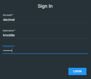
- Click the blue Login button
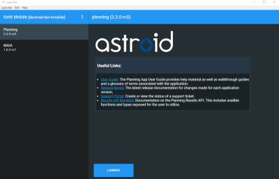
- Select your realm from the list of available realms
- From the left side tool bar select the application you would like to launch
- Click the blue Launch button
- If there is an updated version of this application, the Launch button will not appear and instead an Install button will be available. Click this to allow the latest version to install. After the latest version is installed, the blue button will revert back to Launch, which you can now click
- This will open the Astroid Planning application and bring you directly to the main patient search screen
- You may now proceed with opening a current patient or importing a new patient


Uploading DICOM Patient Files
The Astroid Planning App stores a list of DICOM files (only CT Image Set and Structure Set files are supported at this time) that are available and ready for Import. There are several approaches that can be used to upload DICOM files into this list.
DICOM Receiver Service
For clinical users, a DICOM receiver is generally installed, allowing for direct exporting from contouring software or other planning systems for use within Astroid. In such cases, this DICOM receiver service will be pre-configured to upload the incoming files directly to Thinknode and will also create the records necessary for the DICOM files to be populated into the Astroid Planning App list of available Imports.
Uploading using the Planning App
DICOM files can also be uploaded directly from the Astroid Planning App. The steps below describe the process in detail.
- Open the Launcher and choose the appropriate realm and application to work in
- Choose the Imports block and click the blue Browse button in the Upload Files sub-block
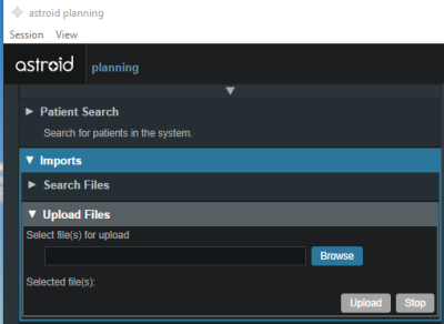
- Navigate to the directory where the DICOM image and structure set files are stored and click Ok
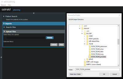
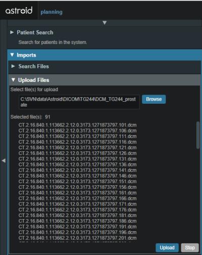
- All DICOM files found in the selected directory will populate in the list field
- If the file list appears correct, click the blue Upload button in the bottom right corner to start the Upload
- This may take a couple of minutes to complete
- Once the file(s) finished uploading they will appear in the list of available files, click back on the Search Files sub-block to return to the list of available files


Bulk Importing using Python
Note: This section requires the user to be familiar with python and the existing .decimal python libraries.
Importing a new patient into the Planning App requires taking a local DICOM directory and posting each of the files through the Dicom App utilizing Thinknode. Each DICOM patient is posted to the Thinknode ISS and an entry is then added to the thinknode RKS that allows the Planning App to see that a new patient has been added. The steps below explain how to upload patient DICOM files using the open source python Astroid Script Library.
- From the .decimal GitHub repository open and edit the post_dicom_patient_rks.py python file.
- Ensure the thinknode.cfg file is set appropriately for your user, account, and realm.
- Edit the following line to point to the directory in which the DICOM patient files are located (note: all DICOM files in this directory will be uploaded):
# Post patient data into ISS
obj_list_id = dicom.make_dicom_object_from_dir(iam, 'F:/Datasets/demo-patient/prostate')
- Run the script and allow the patient to upload to thinknode ISS. After the DICOM patient files are uploaded to ISS, an RKS entry will be created for the Planning App to recognize it as a DICOM file that is available for import.
Importing Patient Data
Now that a patient has been uploaded from DICOM, the Planning App should recognize that new patient files are available to import into a Planning patient.
- Open the Astroid Launcher and launch the Planning App from your realm
- Once Astroid Planning starts, click on the Imports Block in the task control pane on the left side
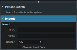
- Select the CT image set from the list of available files for import
- Ensure that the MRN is correct
- Click the Create Patient button to start the import process
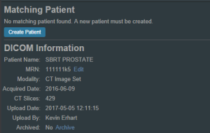
- Ensure that the date and time displayed in Astroid matched the current date and time in the current Windows OS.
- Fill in the requested Patient Intent, taking care to select the appropriate Treatment Site as this selection contains the template information that will be used during structure set import
- Select the appropriate HU to RSP curve (as shown below)
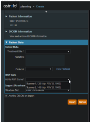
- The corresponding structure set (SS) file to import with these images will automatically be selected. The structures will show up below the Patient Data box in the Import structures box (note that the available choices will be automatically filtered based on the structure set DICOM UID information)
- The structures associated with the data set will be seen in a list of the available structures
- Here you may choose whether or not to import each structure by checking or unchecking the box beside each structure name
- Matched, Assigned, and Custom structures are designated with corresponding tags at the end of the structure name in the structure list
- You may only edit structures that are shown as Custom, which indicates the name did not exactly match a course structure from the Treatment Site template selected above
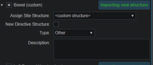
- For all custom structures, the type is by default set to the value from the DICOM file. If there is no type specified in the DICOM file the type will be set to “Other”, unless it contains the letters “TV” (as in PTV or CTV), in which case it is assigned the type of “Target”; the type may be changed here if needed
- Alternatively you may Assign a Custom structure to a course level template structure using the provided drop down menu (this is useful when structure names contain typos or contour names otherwise do not match your standard site protocols)
- Assigning a custom structure to a defined course structure will result in the imported structure inheriting all the predefined structure properties (e.g. name, type, color)
- Once all structures have been selected, assigned, and edited as needed, click the Import button to create the patient and import the CT Images and Structures into it
- The patient is now created and all available data has been imported
- Click on the Back to Import button to return back to the Imports task


Structures in the Data Model
There are multiple levels that various structures can live at. Each level and structure type will effect how the structure will relate to the plan. Refer to the Structure Data Model Guide for more details.
Courses
Overview
The Astroid patient data model uses a hierarchy of items to model the real world workflow patterns of the radiotherapy treatment process. Please refer to the Heirarchy (Data Model) page if you are not familiar with these concepts.
During patient creation (i.e. Importing) a patient record is created containing a Course and a Patient Model. During Import the required data for the Course and Patient Model are entered, however, the Course remains incomplete. The Course will still require physician directive information including the breakdown of the treatment Prescriptions and (optionally) the specification of Clinical Goals. Before creating a Plan this information must be entered. Once the Prescription is complete, plans can be created. The following sections provide a walk through for completing the Course information.
Prescriptions are cumulative. For example: when adding a second prescription, it is assumed that the highest dose from the first Rx has already been delivered to the target for the second prescription. Therefore, the total dose to all targets in the second prescription will have the first prescription's highest dose added.
Completing the Course Prescription
- From the Patient list, select a patient to be opened by clicking the patient row
- The patient will open to the patient overview task and a message will appear telling the user to complete the Prescription information
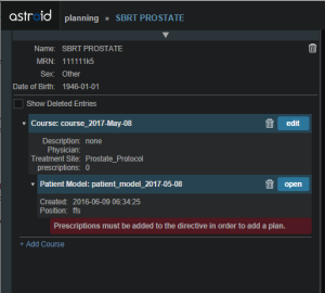
- The Prescription information is part of the Course, which can be edited by clicking on the blue edit button beside the Course label in the patient overview
- The Course Prescription information is mandatory to fill out in order to proceed with planning and at a minimum one Prescription must be created (Clinical Goals are optional)
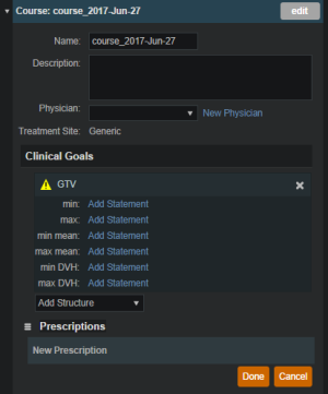
- The Course contains some basic information as well as two blocks of data: Clinical Goals and Prescriptions
- Clinical Goals are used fill in the “goals” (objectives) the physician would like to see achieved by the plan
- To add a goal, simply select click Add Structure and select a desired structure (the choices in the structure drop down will be set by the treatment site template) to which goals should be added
- The user can create goals for tumor volumes as well as Organs at Risk (OAR) and can specify minimum dose, maximum dose, mean dose, and volume based (DVH) goal types
- The Clinical Goals will be used for reporting purposes to describe the physician's intent for the treatment; these do not affect the calculation or plan directly
- The second major part of the Course are the Prescriptions
- This is where the user will fill in the number of fractions and the prescription dose that specified by the physician
- Note that a prescription must be created in order to start the planning process
- Click New Prescription under Prescriptions to create a new empty phase
- The Prescription label and description are free text fields that the user can enter to help identify a particular phase as needed
- If the structure chosen is not contained within the patient model a yellow triangle will appear next to the structure chosen alerting the user
- A color may be selected for the Phase to aid in identification as well
- The number of fractions to be treated should entered and at least one Prescription value must be added (the choices available in the structure drop down will be only the targets from the selected treatment site template)
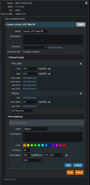
- Once all Prescription information has been entered, click the blue Add button to complete the Prescription
- Additional prescriptions may be added at this point if needed (for example, for a treatment needing a base treatment and a boost)
- The Course should now be complete
- Click on the Done button to return back to the Patient Overview


Patient Models
Once the Course has been completed the next block will be the Patient Model. The Patient Model contains a single CT image set and all contour variants (targets and organs at risk) associated with these images.
About Patient Models
- Patient Model: captures the state (anatomy) of a patient at a certain point in time. Each Patient Models contains a single Image Set (typically CT) and all contour (structure) variants associated with these images. Each unique Image Set imported into the patient should produce a new Patient Model. Each unique structure set imported into the Patient Models should produce new contour variants for each unique contour. Each contour may have only a single “active” variant and the plan will automatically update based on the selection of the active variant.
- Variant: A specific model of a target, OAR, or other structure. A physician may provide an initial target contour and a treatment plan might be generated using this information. The physician may later (using the same CT image set) provide a revised target contour. Rather than import this revision as a new structure or override the original, you may specify this new contour as a variant of the original and the plan will automatically update based on the selection of this new active variant (note each contour/structure may have one or many variants, but only a single variant can be designated as “active”).
Structure Data Model
There are multiple levels that various structures can live at. Each level will effect how the structure will relate to the plan.
Note:
- The assignment of structure type will determine the types of constraints or objectives you can put on the structure.
- Only structures with a Type of Target can be used as Beam Targets
- Site level, Course level and Custom structures can be shared within plans on the same patient
Site Level Structures
Site level structures are predefined templated structures. The user is not allowed to edit any aspect of a Site Level structure. Site level structures may be used for prescriptions as long as they have been designated as a Target.
Course Level Structures
Course level structures are not predefined templated structures (Site Level Structures). Course level structures may have certain properties edited within the planning user interface (e.g.: their type). A structure may be assigned as a Course level structure by choosing the box “New Course Structure” option at the time of import for any structure that does not automatically match a Site Level Structure.  Structures that have been changed to Course level will have be designated as such by the word “course” appearing in parentheses beside the structure name during import. This is useful when a structure was misnamed during the contouring process. Course level structures that have been designated as Target structures can also be used for prescriptions. Any structure with TV as part of its name will automatically be designated as a Course Level structure.
Custom Structures
Custom structures show up at the Patient Model level. These are structures that were not part of the templated structures nor assigned as a Course Level structure. The user has the option to edit the properties of a custom structure from within the Patient Model task. 
Plan Level Structures
Plan level structures are structures created with the Astroid TPS. These structures are derived from existing structures (e.g.: expansions, combinations). See Patient Geometry on how these are created.
Structure Types When Used in Optimization Constraints and Objectives
The structures type determines the options available to the user when specifying constraints and objectives for the treatment plan optimization (refer to Optimization Constraints and Optimization Objectives for definitions of Constraints and Objectives). Below explains the structure types and options available for each type during optimization:
Non-Target Structures
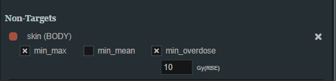
For structure types that are not Target or Other the user only has the ability to set constraints and objectives that drive the dose downward.
- Constraints: only maximum and maximum mean dose settings can be added to the structure.
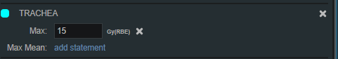
- Objectives: only minimizing objectives (minimize the maximum, minimize the mean, and minimize the overdose) can be added to the structure.


Target and Other Structures
For structure types that are Targets and Other the user has the ability to set constraints and objectives that drive the dose upward and downward.
- Constraints: Both maximum and minimum dose and mean dose constraints can be added to the structure.
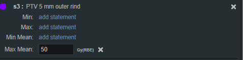
- Objectives: Both minimizing and maximizing dose objectives cab be added to the structure.


Working with Patient Models
Within Astroid the planner has the ability to view the Patient Model details and edit certain structures in a limited capacity.
- A Patient Model contains data relating to the image set such as the number of slices, who imported the image set, the import date and the UID.
- A Patient Model also contains a list of the structures that were imported.
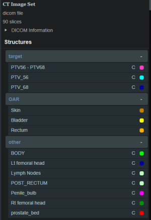
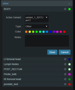
- The user may choose to set the active variant for any structure present in the snapshot.
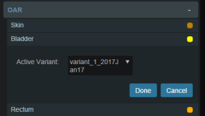
- Structures not defined in the site config (i.e. custom structures) are denoted with a “c” beside it. These structures have the ability to be edited in a limited capacity. The planner may choose to change the structure variant, color, and structure type. The planner may also choose to enter any notes that may be helpful at this point.


Creating a Plan
- The point has now been reached where a Plan can be created
- Click on the blue Add Plan link under the Patient Model to create a new plan
- In the box that opens the user should name the plan and add any description they may want
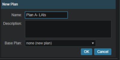
- Note that the Base Plan option is used to specify whether an empty plan should be created or if the new plan should be pre-filled using the selected Plan Template (details on Plan Templates can be found here)
- Click on the blue OK button when finished and the Plan has been created
- Open the plan and begin the planning process by clicking on the blue Open button next to the new plan
- Note that users are free to have as many plans as desired within a the Patient Model and each Plan will specify which portion of the Course Prescriptions it is attempting to implement

Patient Geometry
Patient / External Structure
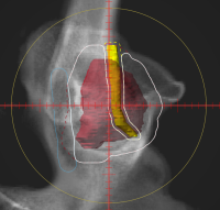
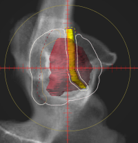
The Patient or External structure is one of key importance in Astroid. This structure is used to define the extents of the dose calculation process. This includes the extents of the dose grid, as well as useful area of the CT images for the purposes of Relative Stopping Power conversion. Planners should be aware that all area outside of the External contour is considered to have an RSP value of 0.001 (air). As a result please ensure that any devices that need to be considered in the calculation such as: patient immobilization or positioning devices or the couch are contoured as part the external contour if they will be present during treatment and may impact the delivery beams. Please note in the example below how the planner included the head holder, mask, and S-frame as part of the External contour so that all of these devices will be included in the dose calculations. The couch was safely excluded in this example because no “through couch” beams were going to be used in this treatment. This “air” override is applied BEFORE any manual user overrides are applied.

Structures
Within Astroid the planner has the ability to create additional structures that may be needed when building a treatment plan. The Astroid Planning App allows for new structure creation using modifications of existing structures only. These modifications include boolean combinations, expansions/contractions, rinds, and clipping (i.e. splitting by a plane).
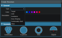
General Structure Options
- Type: Set the type of the new structure (Target, OAR, Avoidance, etc)
- Type may be left blank to allow it to be “inherited” from the type of the base structure
- Color: Display color for the new structure
- Description: Optional, user specified text describing the new structure
Structure Geometry Types
The following is a detailed explanation of each of the structure geometry functions that may be used to create or edit structures within Astroid.
Combination
Allows for the combination of two or more structures using set (boolean) operations. The planner must choose which type of set operation they desire to create the new structure.

- Union - Combine two or more structures. The resulting new structure will contain the points that are within ANY of the selected structures. Structures are selected from a series of simple drop down menus. Refer to this union example for a sample of a union structure being created.

- Intersection - Use only the overlap of two or more structures. The resulting new structure will include only the points that are in ALL of the selected structures. Structures are selected from a series of simple drop down menus. Refer to this intersection example for a sample of a intersection structure being created.

- Difference - Subtract one or more structures from a base structure. The resulting new structure will include the points that are in the first structure but not the others. The base structure is selected from the first drop down. The structures to subtract are then selected from the next series of simple drop down menus. Refer to this difference example for a sample of a difference structure being created.

- XOR (Exclusive OR) - Combine two or more structures with exclusivity. The resulting new structure will include areas that are within an odd number of structures only and will exclude areas that are within an even number of structures. Two or more structures need to be chosen from the drop down to create the new structure. The shaded areas in the examples below show the new structure and demonstrate the XOR functionality. The non-shaded areas would be excluded from the new structure.


Expansion
Allows for creation of a new structure as an expansion or contraction of an existing structure. The base structure is selected from a simple drop down menu. An expansion is performed by entering a positive number for the expansion amount. Conversely, a contraction is performed by entering a negative number for the expansion amount. Structures may be expranded in two dimensions (structure will only expand/contract within its original slice planes) or three dimensions (structure will expand onto other slices as a true 3D expansion). Please note that the resulting structures are still slice based entities, therefore an expansion by an amount less than a single CT slice thickness may not result in the structure expanding out to additional slices. Refer to this expansion example for a sample of an expansion structure being created.

Rind
Allows for creation of a new structure as a thin ring around the surface of an existing structure. The base structure is selected from a simple drop down menu and then both an inner margin and outer margin are specified. Inner margin is the thickness of the ring toward the inside of the existing base structure. Outer margin is the thickness of the ring outside the existing base structure. Negative margins are not permitted, although zero is permitted for either value, allowing for the creation of one-directional rinds. It should also be noted that the resulting rind structures are still slice based entities, therefore rind thicknesses may not be fully uniform at the superior and inferior ends, as contours are limited by the CT slice positions. Refer to this rind example for a sample of a rind structure being created.

Clipped
Creates a new structure by splitting an existing structure by a user defined plane (and discarding the portion on the positive side of the plane). Any existing structure may be selected for splitting from a simple drop down menu. The split plane is defined by a single point and a normal vector pointing away from the portion of the structure that will be kept. The normal vector is defined by its three direction components XYZ and the point may be selected (or created) from the available point list menu. The XYZ normal vector directions refer to patient coordinates so that X is left-right, Y is ant-post, and Z is inf-sup (note: if the “wrong” side of the structure is removed, simply reverse the direction of the normal vector by changing the sign of each XYZ value). Refer to this clipping example of a clipped structure being created.

Working with Structures
This section walks the user through the creation of a of a new planning structure (an expansion structure is used herein for illustration purposes).
- Open the Patient Geometry block
- This will open the patient Structures list
- Click the Create New Structure button at the bottom of the list
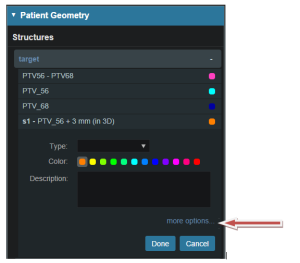
- Next, choose the Type of structure that should be created from the drop down menu at the top (or leave this blank to “inherent” the type from the base structure)
- Change the Color and enter a Description if desired
- Then, select the method of creation desired for the new structure: Combination, Expansion, Rind, or Clipped (see above for details about each method)
- Choose the required structures and enter any other required information for this method and then click Create to complete the new structure
- For this expansion structure, the base structure and the expansion amount are all that is required
- Once a structure has been created, it can be edited, cloned, or deleted by clicking on the structure and then clicking on the appropriate button
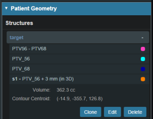
- Note that when editing a structure, only simple options are immediately presented to the user, if further editing of the structure is needed, simply click on more options to open the full structure editing task which allows for editing of all structure options


Points
Within Astroid the planner has the ability to create additional points that may be needed when building a treatment plan. These points include Isocenter, Point of Interest (POI) and Localization points.
General Point Options
- Type: Set the type of the new structure (Isocenter, POI and Localization)
- Type may be left blank to allow it to be “inherited” from the type of the base structure
- Color: Display color for the new structure
- Description: Optional, user specified text describing the new structure
Working with Points
- Open the Patient Geometry block
- Click the Create New Point at the bottom of the Patient Geometry box
- Next, choose the Type of point that should be created from the drop down menu at the top
- Change the point Color and enter a Description if desired
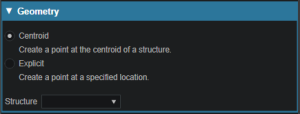
- Next choose the point location- Centroid or Explicit
- Centroid will place the point in the center of the structure chosen from the drop down list at the bottom of the Geometry box
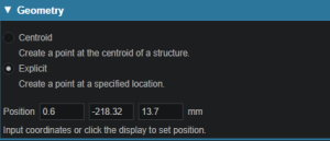
- Explicit allows the user to place a point anywhere within the patient. The user will may enter the point coordinates in the XYZ axis (The XYZ normal vector directions refer to patient coordinates so that X is left-right, Y is ant-post, and Z is inf-sup) or may simply click and drag on a display to select the location of the point.


RSP Image
The RSP Image block allows the user to choose (if not chosen during patient import) or change the HU (Hounsfield Unit) to RSP (Relative Stopping Power) curve to use during the planning process. The user may also choose any density overrides for a particular structure at this point. An example of when to choose an override is the case of hip prosthesis. The user will need to know the RSP to be used for the chosen structure.
- Open the RSP Image block
- Choose the HU to RSP curve (if you wish to override the one chosen at import) from the dropdown list
- If a structure needs a density to be overridden choose that structure from the Add Override dropdown list
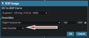
- Enter the RSP value for the chosen structure
- Click OK when done

The order in which density overrides are applied can often be important to users. The Planning App first applies the override outside the “external” structure and then applies any user added overrides in the order added by the user.
Note- Please see patient_geometry as to how RSP outside of the patient external contour is handled
Dose Grid
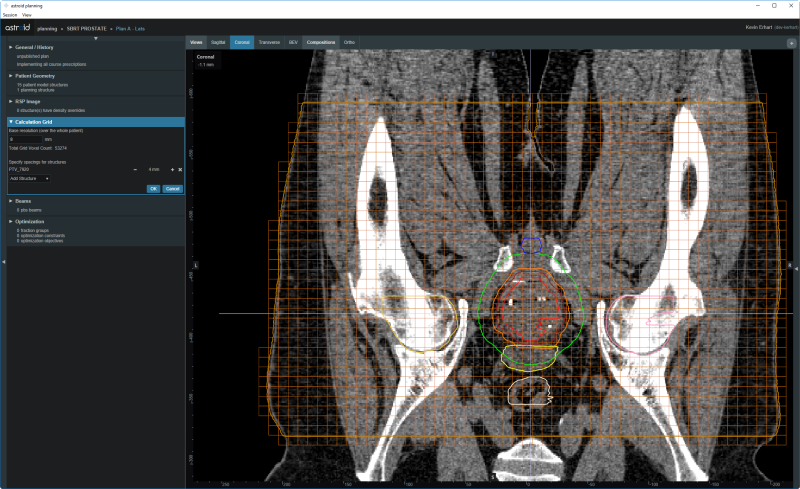
Astroid utilizes a calculation grid that allows for local grid resolution to be specified on a per structure basis. This allows for improved optimizer performance in terms of both speed and resultant plan quality. A uniform sized base calculation grid is created over the entire patient structure. This base resolution can generally be set to a size much larger than the value needed for accurate clinical dose resolution. The user can then reduce the grid sizes in critical areas, generally the high gradient regions and target areas that require homogeneous dose, by assigning appropriate structures a smaller grid spacing value. A common configuration is to use a base resolution of 8mm, 4mm within critical OARs and the PTV/CTV and 2mm in a thin (rind) region surrounding the PTV. This provides sufficient dose information for the optimizer to maintain uniform dose to targets, drive down dose to OARs, and achieve steep dose fall at the boundaries of targets and healthy tissue. An example of constructing such a grid is given below.
- Open the Calculation Grid block
- The default base resolution is set in the site specific configuration settings and is applied throughout the entire patient
- This value may be adjusted if needed
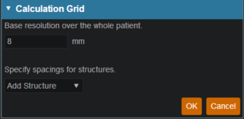
- If you want to use a smaller grid in a target or OAR choose that structure from the dropdown and then specify the desired resolution
- Note that allowable resolutions are scaled down by powers of 2 from the base resolution by using the +/- on either side of the region spacing setting
- Notice the different size grid in the PTV and the patient
- Additional structures with different resolutions may be added, such as for a high resolution dose-falloff region using a rind structure or very small OARs
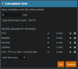
- Once the appropriate regions and resolutions have been set, click Ok to save the calculation grid
- The Calculation Grid block can be revisited at any time to adjust the grid if needed


Proton Beams
Defining treatment beams will be one of the most important tasks within the Astroid planning system. Defining appropriate beams will require users to use their knowledge and experience to properly select many of the parameters that define a treatment beam. These parameters include the target, geometry (isocenter, gantry and couch angles), beamline devices, air gap, and spot placement options. The Beam task utilizes a series of blocks to organize the beam creation process into a common step-by-step sequence. Several blocks are optional as not all beams will use all features. Additionally, it is important to point out that the treatment room & default spot placement parameters are set outside of the individual beam creation tasks as these apply to all beams (however, spot placement parameters can be overridden within each beam if desired). An example of constructing a lateral beam, with the isocenter at the centroid of the PTV is given below to illustrate the features available when defining a beam.
Treatment Room & Mode Type (SOBP or PBS)
- Within the Plan Overview select the Beams block
- From this interface you can select the treatment room, including the treatment mode
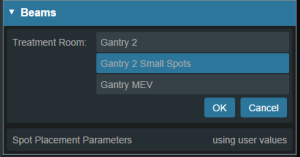
- If the treatment mode is PBS you can then select and define the plan level PBS Spot Placement Parameters. Edit these parameters to define the spot placement grid for each beam in the plan, noting that individual beams can override these values during beam creation if you so desire

Beam Creation
- The next step is to create the beam by clicking the:
- Create New PBS Beam button for use in PBS treatment rooms
- Create New SOBP Beam button for use in SOBP treatment rooms
- Now we will proceed step-by-step through the various “blocks” to create a complete beam as shown below:
General Settings
The General block is used to set general beam details including:
- Color, Beam Label (or select automatically generate label) and Description
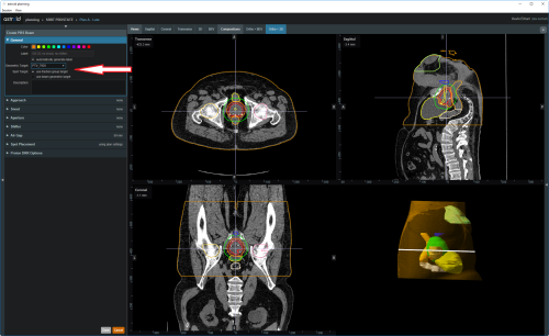
PBS specific
For PBS beams the following additional options will be available:
- Geometric Target is used for approach and device creation. You may choose an existing target or create a new structure. For this example we chose the PTV_7920 as the geometric target. The geometric target will be used to define the extents of the aperture (if used) and will be linked to the isocenter position (if target centroid is selected in the approach block).
- Spot Target is used to define the extent of the PBS spot placements for the beam. The spot target can either match the geometric target, or the user can choose to use the target for the fraction group in which the beam is used (useful for allowing the same geometric beam to be used in multiple fraction groups by simply recomputing the spot positions based on the fraction group target).

SOBP specific
For SOBP beams the following additional options will be available:
- Target is used for approach and device creation, and it can be either a structure or an existing beam.

- If the target selected is an existing beam, the new beam becomes a Patch beam. Thus, the targeted beam becomes a parent thru-beam of the current patch beam (child).
- The patch dose field box is then enabled, allowing users to enter a dose value amount. The parent beam's target will reduced such that any portion receiving a dose from the parent beam that is greater than this amount will be ignored when designing the patch beam range compensator. In other words, the target of the patch beam becomes the target of the parent beam, minus the volume enclosed by the isodose surface (compute only for parent beam) at the defined patch dose value. This patch beam target can be viewed in the Display UI and toggled on and off in the right hand side beam controls.
- Patch beams can also be “chained” beyond a single parent-child pair by creating a beam and selecting the desired patch beam as the target.
- Also note, that once a beam is designated as a patch and added to a fraction group, it cannot be changed back to a standard non-patch beam. In such cases, you must either remove the beams from the Fraction Group first, or a new SOBP beam must be created.
Beam Approach
In the Approach block specify the desired isocenter from the dropdown. You may choose to use the centroid of the Geometric Target (as shown below) or you can select or create a new point to define the location for the isocenter. The gantry angle and couch angles are also entered here as well. Editing these values can be done by typing directly in the provided fields or by using the sliders. The patient in this example is feet first so we will use 90 for the Gantry angle and 0 for the Couch Angle to create a left lateral beam. 
Snout
In the snout block a list of snouts associated with the specified treatment room will be available to choose from. Selecting a snout can change what beamline devices are available based on the facility model in the site info.
Apertures
An option to add an aperture can be found within the Aperture block. An Aperture was not chosen in the PBS beam example. Although selecting an aperture is optional for PBS beam plans, selecting an aperture is required for SOBP beam plans.
- Refer to Creating a New Aperture for detailed instruction
Shifters (PBS)
The Range Shifter block is only available for PBS treatment modes.
- If desired, select the range Shifter to use based on the ones available for the selected snout. If no Shifter is needed as in the example given, the user may go to the next step
Air Gap
Once the beam line devices are defined, we can move to specify the Air Gap distance. The valid air gap range will be listed based on the selected snout. The user may choose any value in this range. 30mm was chosen in the below example.
Beam Spot Placements (PBS)
The Spot Placement block is only available for PBS treatment modes.
- With the beam positioned and any beamline devices put in place, the user is ready view the PBS Spots and adjust the Spot Placement values if needed. The Spot Placement box, if chosen, will allow the user to set new parameters, overriding the spot placement parameters for this one beam if desired. The example below illustrates the message shown when using the spot placement values from the plan level.
Proton DRRs
Proton DRRs do not impact the beam and are used purely for visualization purposes so that you can set the DRR Options to levels that generate appropriate anatomy visualizations. An example DRR is shown below. Note that Astroid allows you to define 2 distinct DRRs and then blend them together using a simple weight factor to create a single DRR image on the screen. This gives users the freedom to create high contrast, high quality DRR visualizations. A single image was used in the example below as the second set of DRR options has the weight set to 0. 
Creating an Aperture
An aperture can be added for any snout that has slabs defined for use in the site specific machine model. The site model also includes a definition for the aperture milling tool and Astroid enforces the “millability” of all apertures so that dose is only computed using a device that exactly matches what will be manufactured. The user has the ability to utilize apertures for all types of proton delivery including: PBS, DS, and US. The major steps involved in creating an aperture are common to all delivery modes, so the PBS beam example below can be referenced for all cases.
Adding an Aperture
PBS
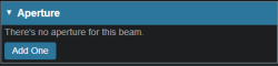
- From within the PBS Beam Task you may add an aperture to a beam by clicking the “Add One” button from within the Aperture Task Block.

SOBP
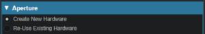
- From within the SOBP Beam Task, an initial aperture is automatically created (note: the “Create New Hardware” option is selected from within the Aperture Task Block) based on your site configuration default margins and the selected beam target. Changes to the default aperture can be made according to the instructions and descriptions below if needed. Alternatively, you can re-use an existing aperture by clicking the “Re-Use Existing Hardware” button. Selecting the “Re-Use Existing Hardware” option ensures that the current beam will use the exact same device used in an another beam within the plan.

Target
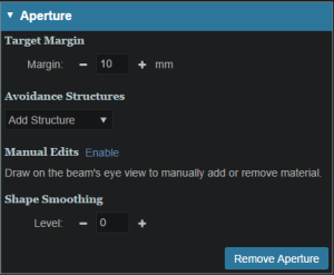
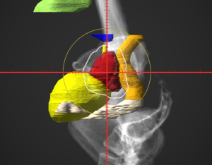
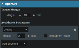
- Your target structure is automatically selected from your beam setup information. So you need to only specify the number of millimeters you want to expand your aperture around the target structure using the “Margin” option to generate your initial aperture shape. For this example we will give a margin of 10mm around the PTV7920.
- Your aperture should now appear in the BEV display window.
- As seen in the example, the aperture is created so that it there is a 10mm margin from the PTV7920 to the edge of the aperture.


Avoidance Structures
- In many cases you may have nearby critical structures that must be avoided. You can add an “Avoidance Structure” to your aperture design by clicking on the “Add Structure” dropdown and selecting a structure.
- Once added you can now specify a margin (mm) around this structure if desired (note negative margins will reduce the size of the blocked area, exposing part of the structure to the open field).
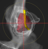
- You may also choose to occlude the structure by the target or not using the “Occlude by Target” option. For the following examples we will use the Urethra as it shows a dramatic example of differences of using or not using the “Occulde by Target” option. A 2mm margin was applied to the Urethra for the following examples.
- By checking the “Occlude by Target” box you are choosing to give the target priority over the structure in the view you are looking at in the DRR. In other words the visible target (target in front of this structure) will not be blocked by the aperture. Note that just the inferior edge of the Urethra is blocked by the aperture. The part of the Urethra that is behind the PTV7920 is not blocked.
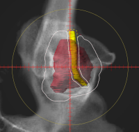
- If you leave the “Occlude by Target” unchecked, you are choosing to give the structure priority over the target. This means you will block the entire structure regardless of its position relative to the target. In this example the aperture blocks out all of the Urethra.
- You may add as many Avoidance Structures as needed to design your aperture shape.


Shape Smoothing
- The “Shape Smoothing” section allows you to smooth the aperture if needed.
- The smoothing level value can be set from 0-20, with zero applying no smoothing and higher numbers increasing the smoothness of the aperture. See dosimetry explanation on aperture smoothing for more details regarding the smoothing algorithm and process.
Manual Edits
- Manual edits allow you to draw on the BEV in order to manually edit the aperture shape. To begin editing simply click the Enable link.
- First, set the radius of the editing tool to the desired size (you can directly type a size or use the -/+ on either side to increment the size)
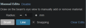
- You are now free to draw manual override regions directly on the BEV. You draw by simply clicking and dragging the mouse at the desired positions.
- You have the option to use a freehand brush tool or a straight line drawing tool for performing manual edits.
- While using the straight line tool, the Snapping option allows snapping for horizontal, vertical, and 45 degree angles.
- The editing tool automatically switches between adding or subtracting material based on the position of the tool when the mouse is first clicked (i.e. when starting each new draw operation).
- When outside the aperture, you edit the aperture by pushing in/subtracting and your edit regions are drawn in a blue color. The hashed red line denotes the original placement of the aperture.
- When inside the aperture, you edit the aperture by pushing out/adding and your edit regions are drawn as the color of your target.
The manual edits contain an “undo” feature, so that the user can successively remove the last manual edit step by pressing Ctrl+Z. Please note that the undo functionality only tracks edits performed in the active session, so as soon as you leave this block or disable manual edits, you will be unable to use the undo functionality on those changes when returning to this task.
- Once done with manually editing, click the “Disable Editing” button to end the process.
- Note that your edits and the resulting aperture shape will still show on the BEV and your edits will remain as-drawn even when changing other options.


Removing Edits
- If you need to remove the manual edits for any reason, you may do so by pressing the “Clear Edits” button. Pressing this button will remove ALL manual edits for this aperture.
Removing an Aperture
- If you wish to remove the aperture from this beam, simply press the “Remove Aperture” button at the bottom of the Aperture Task Block to completely remove it.
Creating a Range Compensator
Note: Range compensators can only be added to SOBP beams.
A range compensator is automatically added for any snout that has range compensator information defined for use in the site specific machine model. The site model also includes the maximum and minimum possible thickness values, the material, and the extents (outer dimensions) of the range compensators for each snout.
Re-using Existing Hardware
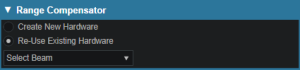
- From within the SOBP Beam Task, you may either create a new range compensator or re-use a range compensator that already exists in the plan. This option ensures that the current beam will use the exact same device defined by another beam within the plan.

Geometric or Dose Based
- Astroid has two algorithms to design proton range compensators, a standard geometric approach and a dose based option. Each is explained below.
- Geometric:
- Ray tracing is used to determine the water equivalent depth (WED) at the distal surface of the target volume throughout the entire treatment field
- Using this data, the appropriate thickness of range compensator material is added to each rayline such that protons will stop at the distal target surface (thickness = r90 - WED)
- This is the standard design approach for range compensators in nearly all other planning systems
- Dose Based:
- This approach begins with a standard geometric design
- Then the actual dose delivered from this field using the current compensator is computed
- Ray tracing is then used to compute the distance between the actual (computed) 90% isodose surface and the distal target surface throughout the entire field
- Material is then added or subtracted from the range compensator for each rayline, based on the difference in depth between these two surfaces
- The process repeats from step 2 for a predefined number of iterations (defined in the site info, and should typically be between 3-10)

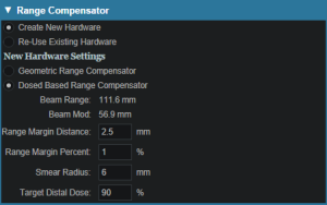
Range Compensator Parameters
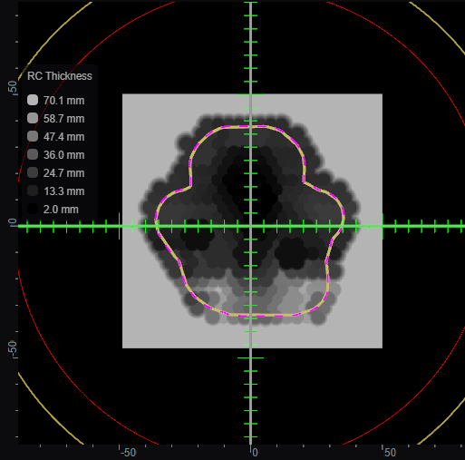
- The range compensator calculation uses a distal range margin that is the addition of the user-defined “Range Margin Distance” and the “Range Margin Percentage” of the beam range. The “Smear Radius” is a distance over which to reduce heights of nearby drill points to avoid narrow valleys in the compensator surface and improve treatment robustness. All drill points are dropped to the lowest height neighbor within this radius. The “Target Distal Dose” is the dose value that the range compensator calculation will try to achieve on the distal edge of the target (most typically 90%).

Astroid Optimization (PBS)
With intensity modulated PBS treatment plans the variety of possible dose distributions is quite large. Typically if a physician does not like a plan they will request it to be re-run. This requires the planner to input new constraints and objectives and a new plan to be run from the beginning of the optimization process. This is a time consuming process. Astroid eliminates this cycle using a Multi-Criteria Optimization (MCO) approach that allows planners and physicians to visualize the trade-offs of target volume coverage vs reduced dose to the OAR's in real time. MCO treatment planning is based on a set of Pareto optimized plans, where a plan is considered Pareto optimal if it satisfies all the constraints and none of the objectives can be improved without worsening at least one of the other objectives. So instead of creating just one plan, Astroid creates a set of optimal plans that satisfies the treatment plan constraints and puts an interactive exploration of the objectives at the planners and physicians fingertips via a unique, highly intuitive, solution navigation slider bar system.
Constraints play an important role in the optimization process, as they bound the solution space and ensure your navigation process is focused only on plans that meet your non-negotiable, highest priority dosimetric needs. It should be noted that if the constraints are too tight, there may be no feasible plans. However, if the constraints are too loose, too many solutions will exist and the navigation will be too broad to provide adequate resolution over the truly clinically useful plans. Therefore care should be taken to ensure appropriate constraints are set, which is facilitated using the Astroid Feasibility check feature. So while constraints supply hard limits, objectives are the negotiable goals, they do not have a hard level that must be obtained, but “pushing” them harder does result in benefit to the patient. The number and type of objectives chosen should be such that all the relevant trade-offs can be demonstrated and explored.
Optimizer Algorithm Selection
The user is able to select the MCO optimization algorithm from a list defined in the site configuration settings. The default option is the first algorithm in this site level list of pluggable_functions designated with the mco_optimizer key.
As of Planning 2.3.2 the available optimizers are Art3+O and Nymph. Both optimizers use the same constraints and objectives. However Nymph does not use a separate feasibility stage and has it built in to the optimization step.

PBS Fraction Groups
Defining Fraction Groups is the first step in the PBS Optimization process within Astroid. Most commonly, a fraction group is simply an arrangement of beams that will be used in a typical daily treatment fraction. The Fraction Group contains some basic group information, as well as Fraction Group level constraints and collections of Beam Sets and Constraints for each target of the fraction group. The Beam Set and various Constraint levels are key concepts within Astroid that allow for high levels of control over the Astroid PBS Optimization engine. Further details of these critical items are provided below and additionally, examples of some common cases and how fraction groups, targets, and beam sets can be constructed to meet the clinical needs of various clinical cases can be found in the Prostate Plan Walkthrough.
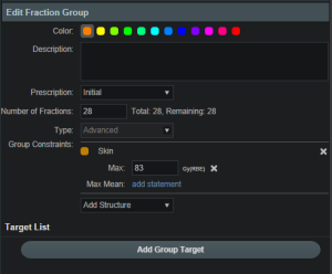
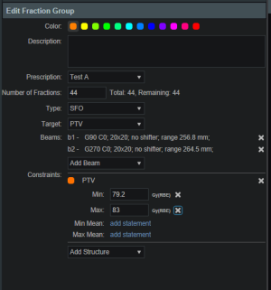
General Fraction Group Data
- Color: Display color of the Fraction Group
- Description: Optional, user specified text describing the Fraction Group
- Prescription: Prescription that the Fraction Group implements; note that only targets containing dose statements from this Prescription will be available when selecting the Target for the Fraction Group
- Number of Fractions: The total number of fractions to be delivered for this Fraction Group; this is very important as it will determine the appropriate Monitor Units for the individual beams
- Type: The delivery approach that will be used for the beams in the Fraction Group. Options for this include SFO, IMPT, and Advanced. If either SFO or IMPT are selected the Fraction Group user interface will remain in “Simple Mode”, whereas selecting Advanced as the type will switch the interface to the “Advanced Mode”

Simple Type Fraction Groups
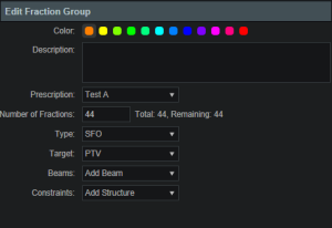
SFO
Single Field Optimized treatments are created using this type option. Simply select SFO from the Type drop down and then add any number of beams and constraints. Each constraint will be equally divided among each beam during optimization. For example, if three beams are included in the Fraction Group and a PTV min constraint of 60 Gy(RBE) is added, then each beam will be individually set to have a constraint of 20 Gy(RBE) (60/3) when running the optimization.
Note: A fraction group with only one beamset and a single beam will always be considered to be an SFO fraction group.
IMPT
Intensity Modulated Proton Therapy treatments are created using this type option. Simply select IMPT from the Type drop down and then add any number of beams and constraints. These constraints will be applied to the collective (total) dose from all beams in the Fraction Group. Using the same example as the SFO section, if three beams are included and a PTV min constraint of 60 Gy(RBE) is added, then the total dose from the three beams must be above 60 at all points within the PTV, however, no restrictions are placed per beam, so that each beam is free to give any portion of the 60 Gy(RBE) dose. This allows for maximum flexibility in sculpting dose to the target, but generally at the expense of increased sensitivity to motion and patient positioning uncertainty.

Advanced Type Fraction Groups
Advanced type fraction groups are needed only in rare occasions when beams must be mixed such that a standard IMPT or SFO approach simply doesn't provide the necessary control over the constraints. Since the advanced more UI is significantly more complex, the following section is dedicated to providing a more detailed understanding of the available options. It should be noted that Advanced mode allows for multiple targets and for constraints to be specified at the Fraction Group level and the Beam Set level and it is important to learn these differences in order to make proper use of the advanced options.
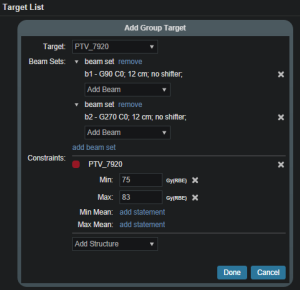
Fraction Group Targets
Simply speaking, a Fraction Group Target is just a collection of Beam Sets and Constraints that together will provide a specified dose to a particular target. In clinical practice, most standard single lesion treatments will use only one Fraction Group Target. More complex prescriptions, such as Simultaneous Integrated Boosts (SIB), generally contain two Fraction Group Targets, one for the primary target and a second for the boost target. Within the Fraction Group Target, a target structure is specified along with one or more Beam Sets and any beam set level constraints necessary to meet the clinical goals for this target.
- Target: The target structure for the beam sets that will be defined below. The available selections will only contain targets with prescriptions specified for the phase selected in the main Fraction Group and that also exist in the treatment plan (note this excludes Directive level structures with prescription information, but no physical contour data).
- Beam Sets: A list of Beam Sets that will be used to achieve the specified constraint doses (see below for a more detailed definition of a Beam Set).
- Constraints: These Beam Set Level Constraints are split evenly and applied individually to each Beam Set
- In other words, the Constraint dose is divided by the number of Beam Sets for the Target, so that both SFO and IMPT can be achieved
Beam Sets
The Beam Set is the lowest level unit for the Astroid PBS Optimizer and proper arrangement of the beams within a beam set allows for both Single Field Optimized (SFO) and Intensity Modulated Proton Therapy (IMPT) fields to be included within the same fraction. A careful review of the Beam Set Level (BSL) Constraints described above, should reveal how to properly arrange beams within Beam Sets to achieve a desired type of treatment. Since BSL Constraints are equally split and are then applied individually to each Beam Set, SFUD beams can easily be achieved by placing each beam in its own Beam Set. Conversely, IMPT beams are created when multiple beams are included within a single Beam Set. Further details of these two cases are presented below, as this will provide the information necessary to allow users to construct complex constraint relationships, which is the purpose of the Advance type UI.
SFO Beams
Single Field Optimized treatment beams are produced by including each beam in a separate Beam Set. This is best understood by example. Suppose a target is intended to receive 20 Gy (2 Gy per day for 10 fractions) from a two beam Fraction Group using a SFO approach. This is achieved by specifying a min dose of 18 Gy and a max dose of 22 Gy using Beam Set Level Constraints. Now two beam sets are created, each containing a single beam, as shown below. Since the BSL constraints are split between the beam sets, this actually tells the optimizer that each beam must provide a min dose of 9 Gy and a max dose of 11 Gy (1/2 of the BSG constraint doses). Therefore, each individual beam will be providing coverage to the entire target as is expected for a SFO approach.

IMPT Beams
Intensity Modulated Proton Therapy treatment beams are produced by including all desired beams in a single Beam Set. This is again best understood by example. Suppose a target is intended to receive 20 Gy (2 Gy per day for 10 fractions) from a two beam Fraction Group using an IMPT approach. This is achieved by specifying a min dose of 18 Gy and a max dose of 22 Gy using Beam Set Level Constraints. Now one Beam Set is created, containing both beams, as shown below. Since there is only Beam Set, the BSL constraints will be applied to the combined dose from the two beams. Therefore, there are no guarantees regarding the uniformity of dose from either beam and instead there is simply the guarantee that the combined dose from the two beams meets the given constraints, thereby producing an IMPT treatment approach.

By understanding the notion that Beam Set Level Constraints are equally split among the Beam Sets, it can also be seen how SFUD and IMPT may be mixed within a Target and even the most complex of treatment scenarios can be handled seamlessly in Astroid.
Working with Fraction Groups
- Select the Create New Fraction Group button
- In the newly opened block the planner will:
- Choose the color the fraction will be denoted in
- Type in any descriptor that may be needed
- Select the phase that the fraction group is implementing
- Enter the total number of fractions to be treated
- Enter the group constraints if desired
- Group constraints apply to the total dose from the whole fraction group
- Constraints for multiple structures may be entered at this stage
- Click Add Target
- Select the target structure
- Create any Beam Sets that are desired
- There may be multiple Beam Sets associated to a target to construct SFUD or IMPT beam groupings (see above for further details)
- Enter any desired Beam Set Level constraints
- The constraints chosen at this point will be evenly divided and applied separately to each Beam Set (see above for further details)
- The user may also have multiple Targets, with each associated to a distinct target within the selected Fraction Group Phase


Optimization Constraints
About Constraints
Constraints can be specified at various levels (Plan, Fraction Group, Target/Beam Set) with Astroid and they will affect different groups of beams depending on their level. Constraints at the Plan level are applied to the total dose resulting from all beams. Constraints at the Fraction Group level are applied to the total dose resulting from only the beams in the current Fraction Group. Constraints at the Target/Beam Set level are split evenly and applied individually to each Beam Set. In other words, the Constraint dose is divided by the number of Beam Sets in the Target, and this dose is then applied as a constraint to each Beam Set, so that either SFUD and IMPT can be achieved (see Fraction Groups). The section below will provide a walk through of the different levels and how constraints are applied at each one.
It should be noted that all constraints are considered “hard limits”- values that must be achieved. Constraints drive the feasibility calculation- whether the plan is achievable and should be used to ensure certain minimal clinical parameters are met.
The following constraint types are available. Note certain constraints are available only for Target type structures.
- Min: The minimum dose the structure must receive
- Max: The maximum dose the structure may receive
- Min Mean: The minimum mean dose a structure must receive
- This will drive the dose up across the structure
- Max Mean: The maximum mean dose a structure may receive
- This will limit the mean dose across the structure
- Overdose: The maximum sum of the overdose that a structure may receive (not available for ART3+O optimizer)
- This will limit the total volume-weighted overdose (dose above a given threshold) that a structure receives, driving down hot spots
- Underdose: The maximum sum of the underdose that a structure may receive (not available for ART3+O optimizer)
- This will limit the total volume weighted underdose (dose below a given threshold) that a structures, driving up cold spots
- Hot Spot Vol: The maximum mean dose to the hottest portion of a structure (not available for ART3+O optimizer)
- This will keep the mean dose to the hottest portion of a structure below the given limit; portion is set as a % vol and the limit is the max mean dose allowed to that portion of the structure
- Cold Spot Vol: The minimum mean dose to the coldest portion of a structure (not available for ART3+O optimizer)
- This will keep the mean dose to the coldest portion of a structure above the given limit; portion is set as a % vol and the limit is the min mean allowed to that portion of the structure
The user can choose to apply one or multiple of these constraints to any number of structures.
Working with Constraints
Working with Fraction Group and Target/Beam Set Constraints
Constraints at the Fraction Group level are applied to the total dose resulting from only those beams in the current Fraction Group. Constraints at the Target / Beam Set level are equally split among the Beam Sets within the Target and are applied to the total dose resulting from the beams in each of the Beam Sets. The following steps are a brief walkthrough for creating a max constraint of 79.2 Gy(RBE) to the PTV for the whole Fraction Group, and then creating two SFO beams that each provide a minimum dose of 39.6 Gy(RBE). Note that this configuration with the max constraint at the Fraction Group Level is different than if we had put both the min and max at the Target / Beam Set level. In the case shown, it is only the total dose from the two beams that is constrained to be below 73 Gy(RBE). Had both constraints been placed at the Target Level, then each beam would instead be constrained to a max of 36.5 Gy(RBE).
- Select the Fraction Group if it has been created or create a new one by clicking Create New Fraction Group
- Choose the prescription, number of fractions to be treated with this Fraction Group
- Choose the type of treatment (SFO, IMPT, Advanced) and target
- Choose the Beams to be treated
- Choose the Target to be treated
- Assign the dose constraints to the Target
- The assigned constraint doses at this level will be divided evenly among the Beams to the Target, which allows for quick creation of SFO treatments


Working with Plan Constraints
Constraints at the Plan level are applied to the total dose across all beams.
- Open the Constraints sub block contained in the Constraints/Feasibility block and choose the Edit button.
- Choose from the drop down the structure or structures to which constraints should be added
- Define what constraint(s) should be applied to each structure by choosing the constraint and entering the dose
- Follow this and enter the constraints for all applicable structures.
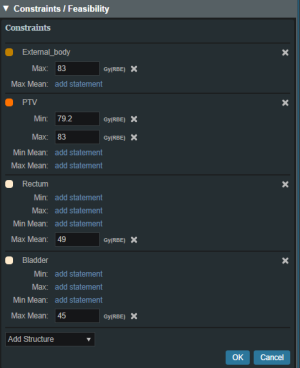
- When finished click the OK button.
- Once all the Constraints have been set the user can either start the Feasibility by choosing Calculate or move on to defining the Objectives

Feasibility and Constraints
After the Constraints have been entered, the user may start the Feasibility calculation by clicking calculate in the Feasibility block. The Feasibility calculation is based solely on the constraints and, it should be used to ensure that it is possible to meet the specified constraints. The Feasibility calculation may be an iterative processes in order to get appropriate constraints established for a particular plan. In other words, the user may need to enter one or more constraints, check the feasibility, then progressively tighten the constraints and re-check the feasibility until the plan is no longer feasible, then back-off to the last feasible values. It is recommended practice to start by obtaining a feasible plan utilizing only target Constraints then add OAR Constraints as desired. Remember, using a narrow range of constraints can improve the optimizer performance and improve the resolution of the solution navigation.
The user also needs to be aware of the impact of Constraints being set at the Fraction Group level versus the Plan level. For example, it is possible to have a Constraint set in the Plan level so that the whole dose to an OAR is given on one day and none on the other day. This could happen when there are two Fraction Groups and the OAR dose is not split between the two by using Fraction Group level constraints.
Optimization Objectives
Objectives communicate to the optimizer the goals that are important to strive for in your plan. Objectives are set at the Plan level under Plan Constraints/Objectives and they apply to the total, combined dose from all beams. Objectives are not given any relative importance at this point (i.e. their order within the list is not meaningful). The Objectives drive the solution of the Multi Criteria Optimization (MCO) and for each Objective, a corresponding Navigation Slider will be presented to allow for exploration of trade-offs in the case of competing objectives (for more information about the MCO process and how objective importance/weighting is handled in Astroid refer to this article).
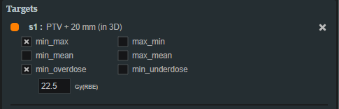
The following objective selections are available in Astroid:
- min_max: Minimize the maximum dose within a structure (drive dose down)
- max_min: Maximize the minimum dose within a structure (drive dose up)


- min_mean: Minimize the mean dose within a structure (drive dose down)
- max_mean: Maximize the mean dose across the structure (drive dose up)
- min_overdose: Minimize the high dose within a structure
- Dose will be driven down only until the specified limit is reached (this is often more relevant that min_max, since it may not be beneficial to continue minimizing beyond a certain dose level)
- min_underdose: Minimize the low dose within a structure
- Dose will be driven up only until the specified limit is reached (this is often more relevant that max_min, since it may not be beneficial to continue maximizing beyond a certain dose level)


- min_hot_spot: Minimize the mean dose to the hottest portion of a structure (not available for ART3+O optimizer)
- The mean dose to the hottest portion of a structure will be driven down (i.e. the tail dose on the DVH); portion is set as a % vol of the structure
- min_cold_spot: Maximize the mean dose to the coldest portion of a structure (not available for ART3+O optimizer)
- The mean dose to the coldest portion of a structure will be driven up (i.e. the shoulder dose on the DVH); portion is set as a % vol of the structure
Working with Objectives
- Open the Objectives/Optimizer sub-block contained in the Optimization block
- Choose a structure to which you wish to apply objectives
- Check the boxes to activate the desired objectives for the structure and then set the dose level if applicable

Once all the Objectives have been set, the user is ready to run the MCO solver, which is performed in the Objectives/Optimizer block.
Running the Optimizer
The Objectives, as stated before are the negotiable goals where there may be no hard limit, but there is benefit to improving them. Astroid allows Objectives on both Targets and OAR's. Objectives can be placed on structures to either increase or decrease dose. The Objectives are the sole driving force guiding the MCO and it is important to recall from the discussion above that Astroid will only navigate to plans that are “optimal” in at least one objective (meaning again that this objective cannot be improved without another objective getting worse). Unlike Constraints, Objectives should be added all at once and there is no need to place them in any particular order (order is irrelevant). Additional information about Objectives can be found here. Since the MCO is finding a large set of optimal solutions the optimization can be a lengthy process. The following factors have the largest impact on the optimization run time:
- The number of points in the calculation grid
- The total number of spots from all beams
The number of calculation points and number of spots will have a direct impact on the calculation times meaning that increases in these values will also increase the MCO calculation time. The number of objectives does not always increase the overall run time of the calculation however, thanks to the parallelization that be achieved using the Astroid cloud services, though the number of objectives does impact the usable capacity of calculations that can run on the Astroid cloud. The speed and number of running calculations will depend on the availability and load on the Astroid cloud calculation servers. Each objective of the MCO calculation is computed on a separate thread of a calculation server, therefore understanding the usage of these servers can help users make decisions regarding resource usage for a given set of objectives. The Astroid MCO calculations are designed to use servers in CPU increments of 16 and the MCO calculations are posted to calculation servers as follows:
- 1-16 objectives: a single 16 core calculation will be issued, with an objective being run on each core
- 16-32 objectives: a single 32 core calculation will be issued, with an objective being run on each core
- >32 objectives: a single 32 core calculation will be issued, and the server will be responsible for balancing the load to achieve full CPU utilization
Understanding this pattern is important, as it can be seen that using less than 16 objectives generally will have minimal impact on MCO run-time and no impact on resource usage. Using between 17-32 objectives will use additional resources, but generally not impact run-time, but using >32 objectives will increase the MCO run-time without using additional resources.
Once all the desired Objectives are entered the MCO calculation is started just by clicking the calculate option in the Navigation block. It should be noted that the Feasibility will be re-checked if any of the Constraints have changed since the feasibility was last run. The MCO calculations will run in the cloud and the user can simply leave the Astroid application running and move on to other things while the calculations process. Please note that at this time the Astroid App should be left open in this state to ensure the calculations run to completion, however, users may open additional instances of Astroid and work on other plans while these calculations proceed (no performance issues should be encountered when using multiple instances since the “heavy” calculations are off-loaded to the cloud calculation servers).
During the calculation process the user may check to see the status of the calculations. The example below shows a Feasibility calculation that is 4% complete. As calculations finish the user will notice this number increasing.  By clicking on Show Details a detailed list of what calculations have been finished and which are running will be displayed. In the example below the dij's are completed and the Feasibility is currently running. In the detailed view if the user chooses show completed subcalculations they will be able to obtain the identification number of each calculation.
Dose Normalization and Display
The user has many options for how the dose is displayed in Astroid. The options for controlling the display of the dose are on the right hand side of the display under Dose Options. The Dose Options provide controls over the DVH type (relative or absolute volume), the colors and scaling of the display dose, the type of dose display shown (colorwash, isolines, or isobands), as well as the scope of dose to display (full plan, single fraction group, or individual beam dose).
Dose Volume Histogram (DVH)
Relative and Absolute DVH
The planner has the option of viewing the dose for the DVH in relative volume (dose per percentage of the volume) or in absolute volume (dose per cc of the structure) using the Absolute DVH option. The user may also hover over any area of the DVH curve to obtain the dose and percentage of a given structure or click on one or more lines to start tracking the cursor value for the lines.


Dual Dose DVH
The planner has the option of viewing the original MCO dose and the currently navigated MCO dose in the DVH graph. By selecting the Show Secondary Doses option under the Dose Options, the DVH graph will display the following doses:
- Dotted Line: Original un-navigated dose.
- Solid Line: Current navigated dose based on the position of the MCO sliders.
With the Show Secondary Doses option disabled, only the current navigated dose will be displayed within the DVH graph.

Dose Display Normalization
As in the DVH the user has multiple options for displaying the dose. The user may change the percentage isodose line and its corresponding Gy they would like displayed. This is done by entering the appropriate numbers in the boxes under Levels. The user may turn on and off specific levels by clicking on the X to the left of the line.
The user also can choose to view the dose as either isobands, isolines, color wash or combinations of these. The user may use the sliders to set the opacity for each of these as well. They may choose the line width and whether it is solid, dashed or dotted for isolines.

In the case of a plan with multiple Fraction Groups the user may choose to view the dose:
- In a composite dose- Full Plan- which will take into account all Fractions groups
- For a particular Fraction Group or
- For an individual beam
To pick one of the above the user must choose from the dropdown list under Scope. The Scope automatically defaults to Full Plan. 
Note: When in a sliced image display containing dose, slice scrolling positions will be based on the smallest voxel size of the calculation grid. For any sliced image displays that do not show dose, scrolling positions will be based on the CT image slice thicknesses directly.
Isobands
Isobands are an interpolation of dose from isodose line to isodose line. Isobands take a range of interpolated dose and fills it in with color.

Isoline
Isolines display either the absolute or relative dose in the form of closed lines of constant dose value (i.e. these are lines that pass through the points of equal dose).

Color Wash
Color Wash shows the raw dose across the given range of values, blending colors according to the dose levels.

Combination
The user does have the ability to combine multiple representations. Below shows a combination of Isobands and Isolines.

Navigating the Solutions
Once the plan has been calculated the Navigation block will become active. This block contains entries for all the active objectives and under each objective is a slider bar. This slider bar allows the user to adjust the importance of an objective and to see, in real time, how the change will affect the dose to the patient.
The Navigation Sliders should provide an intuitive process for finding the optimal plan, but by gaining a complete understanding of the Navigation Sliders users will be better equipped to quickly reach their plan goals. It should also be noted that sliders for minimize objectives will slide to the left and sliders for maximize objectives will slide to the right. On each slider there are two vertical bars. The thick white bar is the user controlled slider handle and it represents the worst value of an objective that the user wants to allow. Simply stated, the objective will not go past this limit. The thin blue bar denotes the actual current value of the objective. Astroid calculates this value by balancing the solution over the available ranges of each objective. It should now be clear that moving a slider does not directly set an objective, but rather it places limits on the allowable range of an objective. It is this feature that makes navigating the solution space very clear and effective.

The blue and white numbers to the upper right of each slider correlate to the objective value for the current plan and the objective limit based on the slider position, respectively. So in the image above, it can be seen that the top slider has been set such that allowable maximum dose to the CTVbreast_L is 10.46 Gy(RBE), but the current value is 10.33 Gy(RBE). The numbers at the end of each slider bar denote the overall range for the objective value (i.e worst and best possible values). The main slider horizontal bar is also separated into two sections. The thicker, lighter grey horizontal bar is the range or window that the objective is currently limited to stay within (it is limited due to the positioning of all sliders by the user). The user will notice as they drag the slider handle (white bar) on one objective, this light grey area will change on some of the other sliders. This allows the user to know the limits they have to work in and the impacts (trade-offs) that one objective is having on the others. Sliders should be adjusted such that all physician goals are achieved and the best balance of target coverage and normal tissue doses are realized for the unique patient at hand.
All of these adjustments are able to be done without running a new plan as would needed to be done in traditional treatment planning systems. This allows the user to look at many different solutions in a short amount of time.
If the user likes the adjustments that were made to the sliders they may click the Save button in the bottom right hand corner. This will save the objectives at their current position. If the user does not like the adjustments they have made to the sliders, they may hit the Reset button to reset all the objective sliders to their last saved state. The Cancel button will close the Navigation block in its current state.
Beam Delivery (SOBP)
SOBP Fraction Groups
Defining Fraction Groups is the final step in the SOBP planning process within Astroid. A fraction group is simply an arrangement of beams that will be used in a typical daily treatment fraction. The Fraction Group contains a list of beams where each beam can be weighted and normalized based on the needs of the patient at hand. Beam normalizations allow for minor field independent adjustments of dose and these factors are limited to stay within 0.90 - 1.10. Beam Weights established the relative fluence of each beam within the fraction group and therefore the sum of the beam weights in each fraction group must be 1.0. Further details of defining fraction groups are provided below.
- To get started, navigate to the Beam Delivery block and click Create New Fraction Group.

General Fraction Group Data

- Color: Display color of the Fraction Group
- Description: Optional, user specified text describing the Fraction Group
- Prescription: Prescription that the Fraction Group implements

- Number of Fractions: The total number of fractions to be delivered for this Fraction Group; this is very important as it will determine the appropriate dose to be delivered from this fraction group, which when combined with the beam weights, provides the proper Monitor Units to be delivered for the individual beams

Beam Options
- Select the beams to be added to this fraction group from the drop down list. Repeat this process as necessary. Notice how one of the beams in the image below is grayed out. This means that the beam has already been selected or it is a patch beam. If it is a patch beam, the beam will automatically be added with its parent beam. There is also the option to create a new beam from the drop-down list.

- Change the normalization factor (if desired) by clicking its box and entering the value desired.
- This is independent from the weight values
- Available as an option for patch beams
- Useful when adjusting hot or cold areas where beams treat the same area or meet
- Weight each beam by either sliding the slider or clicking on the weight value box and typing in the value.
- The value of all beams listed MUST add up to 1.0 (100%)
- By default, the beams are automatically weighted evenly, and, if edited, can be reset by clicking the weight beams evenly option.
- Use the Beam Lock (not available for patch beams) to restrict a beam from automatically adjusting when another beam's weight is adjusted. This option is useful to secure one beam's weight while adjusting the other beams' weights (see image below). The sum of all weights still must equal 1.0.

- When finished, click the Done button. Clicking the Cancel button will reset the changes made to the current fraction group and return the Beam Delivery block to its previous state.
- Repeat this process of adding fraction groups until all remaining fractions are completed.
Plan History
Since the Astroid system captures and stores the user inputs (rather than the results), it is able to maintain an exhaustive history of all edits made to your data with relatively low storage needs. Users are able to benefit from this information through the Plan History feature that is available within each treatment plan. The Plan History is a feature that allows the user to see and explore all the changes and modifications made to a plan. Each modification to a plan will result in a new Revision of the plan (note: in a complex plan there may be hundreds of revisions). If the user is not satisfied with the results of a modification they may go back to any of the previous revisions and restore it to the active instance (note: this will cause another Revision to be created for the reversion). Below is a walk through and more detailed explanation of this feature.
- Open the General block from the Plan Overview and the History item can be seen at the bottom of this block
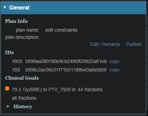
- The summary of the latest revisions will appear in the right display pane
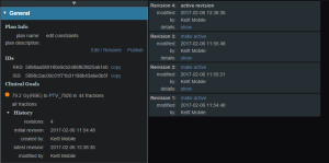
- Expand the History details by clicking the small arrow (this is not mandatory)
- The number of plan revisions will be listed (In the above example there are 4 revisions)
- The user can now review the various revision summaries
- Clicking the blue show link will expand that particular version of the plan and explain what was changed
- “op”: is the operation performed in this version that differs from the previous version (e.g. insert: an item was added)
- “path”: is the item in the treatment plan data that had the operation performed (e.g. points: a point geometry was changed)
- “val”: is the value of the data that was changed (see image below for the “val” of an added point)
- If the user would like to return to this version they may do so by clicking the blue make active link
- The user can close the expanded version by clicking the blue hide link
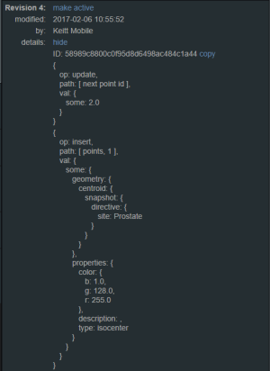


Plan Publishing
Once a physician has approved a plan it should be Published. Publishing a plan allows the user to lock the plan. This means that once a plan has been Published no changes may be made to that plan. A plan that has been Published will be available to “view only”. The Plan History will show the date and time a plan is Published as well as the user who Published it. A plan may not be changed or archived once it has been Published. If a user needs to make a change to a Published plan they will need to copy the Published plan in order to do so. Once the Published plan is cloned they may proceed to make any changes desired.
The following steps outline how to publish a plan in the Astroid Planning App:
- Open the General/History block from the Plan Overview
- Select the Publish button
- You can edit the Plan name and description at this time if needed
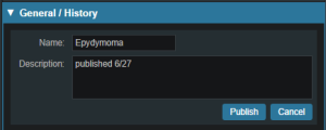
- Once the information has been filled click the Publish button
- The plan will now be denoted as Published in the Patient Overview and users will only have the ability to view or clone the plan
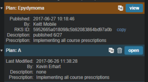


Displays
This section contains general information regarding the various displays available in the Astroid Planning Application. During most tasks, there is a top bar that contains a list of available single and composition views. In most instances these include standard two dimensional sliced views: transverse (axial), sagittal, and coronal. Additional common views include: three dimensional view, Beam's Eye View (BEV), and Dose Volume Histogram (DVH) View.
Beam's Eye View
The Beam's Eye View is a projection of the three dimensional beamline and patient structures into a flat plane as viewed from the beam's proton source. Since certain proton machines may not have a single source point, the BEV supports a dual source projection process as described for aperture devices in the following article, but this is equally applicable to all patient and beamline entities. All projection for the BEV are done to the isocenter plane, therefore all distances measured within the application in the BEV are as projected to isocenter.
Plan Templates
Plan Templates are a powerful feature of Astroid that can greatly reduce the time spent in creating high quality treatment plans. In a simple sense, a Plan Template is just a starting point that can be used when creating new treatment plans for this or other patients. When a Plan Template is applied during new plan creation (see here for creating a new plan), all user specified plan parameters from the template are copied into the new plan. In essence you are applying the plan to a new set of images and structures, therefore it is important that structure names and other data are consistent in your Patient Models when using Plan Templates.
Saving Plan Templates
Plan Templates can be defined globally at the site level for all users at your institution and each user is also free to create their own private list of user level Plan Templates. A Plan Template can be easily created from any existing plan by opening the General/History block. At the bottom of this block the user may then choose either Save as User Plan Template or Save as Site Plan Template. The user then provides name for the Template and fills in any description information as desired.
When saving an existing plan as a template, there are a few rules/tips that should be kept in mind which will help make your templates easier to use in the future:
- In order for templates to work well there needs to be consistency in use of structure names (e.g.- Brainstem consistently labeled Brainstem, not brainstem, Brain stem, brain_stem etc.). Note that proper and consistent use of Site Structure Templates is a great way to ensure this is adhered to by all users.
- Most Astroid Plan parameters reference data that will change properly when applied to a new Patient Model using a Plan Template, however, care should be taken when using Explicit Points as these include fixed coordinate values that they may not transfer as desired from plan to plan. avoiding the use of Explicit Points is the best practice for Plan Templates, but if they must be used be sure to check each explicit point in the new plan after applying a template.
- Plan Templates are specific to the Site Structure Template used by the Patient Model; therefore if a template is created for a prostate patient, for example, that template will not show up for a breast patient due to the Site Structure Template selection being different.
- Keep in mind that a Plan Template can be created to any level of completion desired within the planning process. For example, a simple template could be created that adds only a few planning structures (e.g. rinds, expansions, etc) or a complex template could be saved that includes all plan data including the full optimization constraints and objectives. Different disease sites may lend themselves to different levels of detail in the Plan Template so users are encouraged to explore different options to determine what works best for their clinical workflow.
Using Plan Templates
Plan Templates are applied when creating a new plan:
- Click on the blue Add Plan link under the Patient Model to create a new plan
- From the Base Plan drop down menu choose the Plan Template that should be used and then click OK
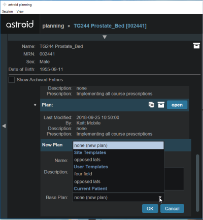
- Open the new plan and check that all plan parameters have been applied as expected (pay special attention to explicit points as described above)
- Make any changes necessary within plan and then proceed with planning from this starting point
- If used well, you should be able to review the plan, make a few minor edits, and be at the point of running feasibility & optimization much faster than when starting from scratch

Plan Export
The Export Block is available in Astroid to allow for saving patient and plan information in DICOM file format. Typically this feature is used once a plan has been completed, the physician has approved the plan, and the plan is ready to be sent to the Record and Verify system for QA and then patient treatment. The process of exporting files and the options available to the user are described below.
- Open the Export block.
- If the plan is unpublished (unapproved), then a qualified person must authorize the export of this plan by checking the appropriate check box in order to perform the export
- The user can choose from the following items to export:
- RT Structure Set
- RT Ion Plan
- RT Dose
- Plan (total dose for all fraction groups and all sessions)
- Fraction Group (dose for all sessions of a single fraction group; each fraction group is exported to its own file)
- Beam (dose for a single session from a single beam; each beam is exported to its own file)
- The export location is then set as either a local directory or to a DICOM server (AE title)
- If exporting locally the choice to anonymize the data can be made by checking the Anonymize patient data box option as shown

- When exporting to a DICOM Server, several options are available
- Preset AE Titles which are managed through the Site Configuration can be selected or the custom option is available in which a specific server name, location, and communication port ID will need to be specified
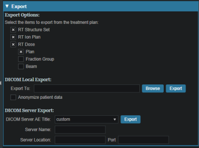

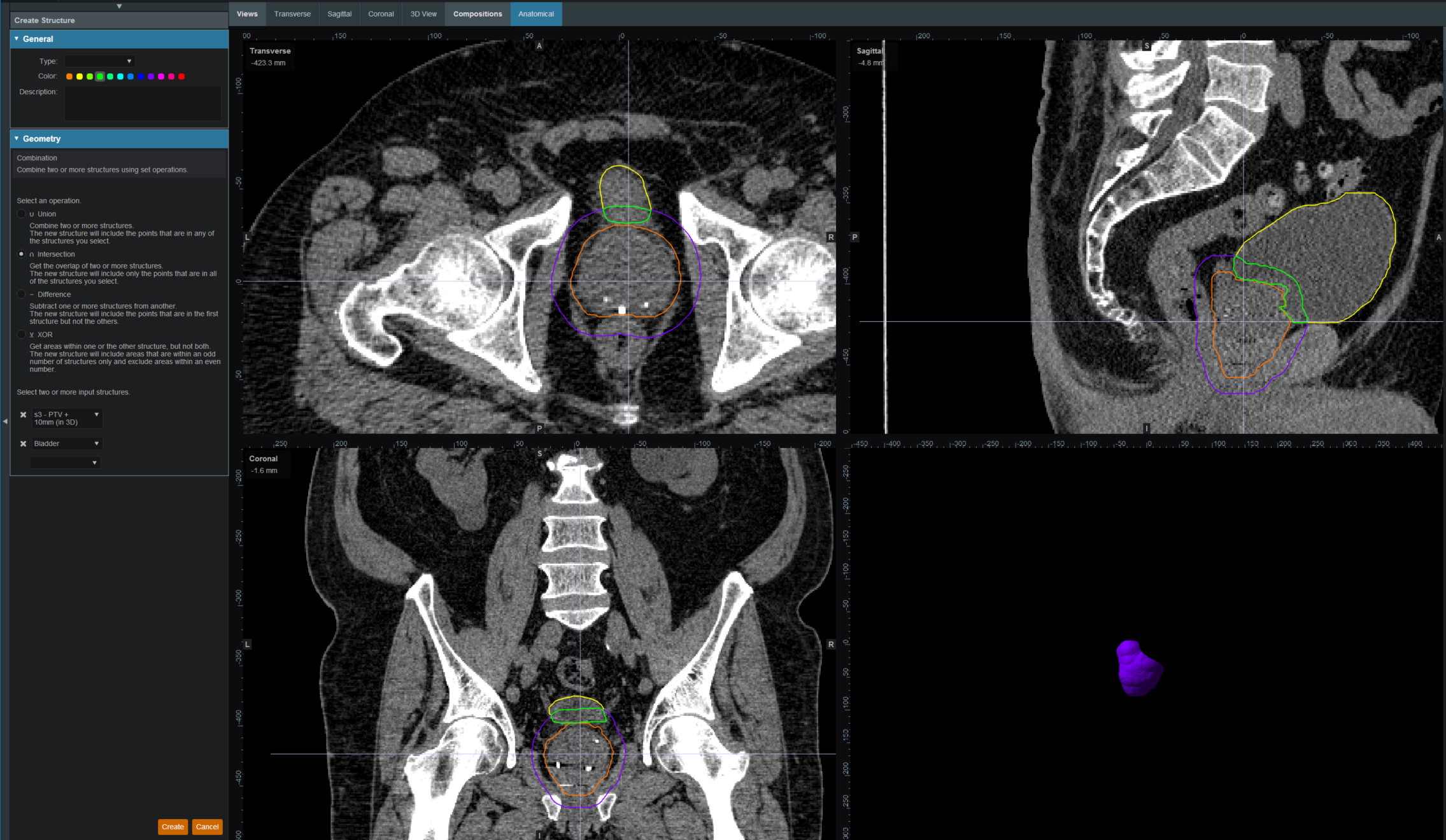
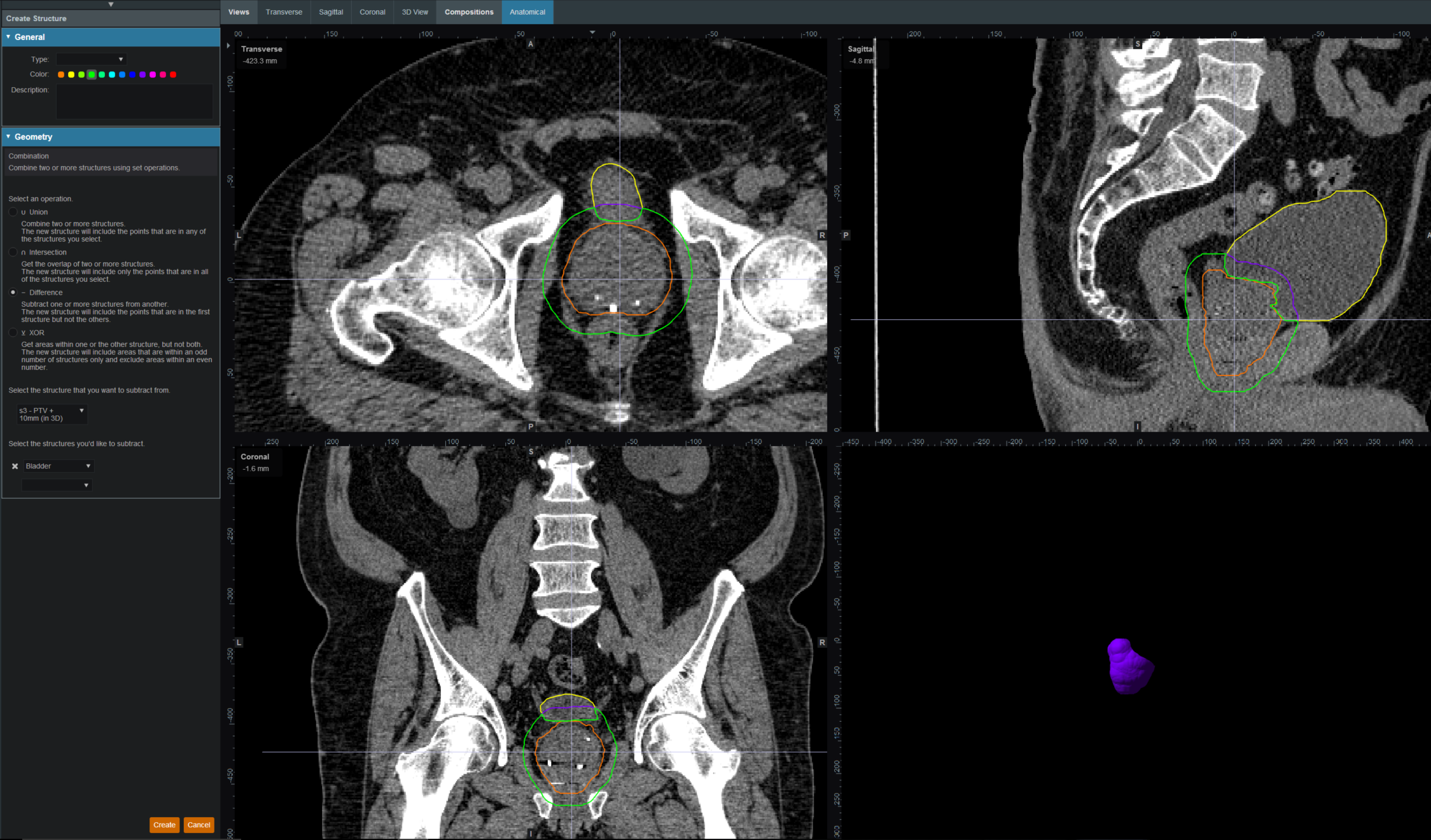
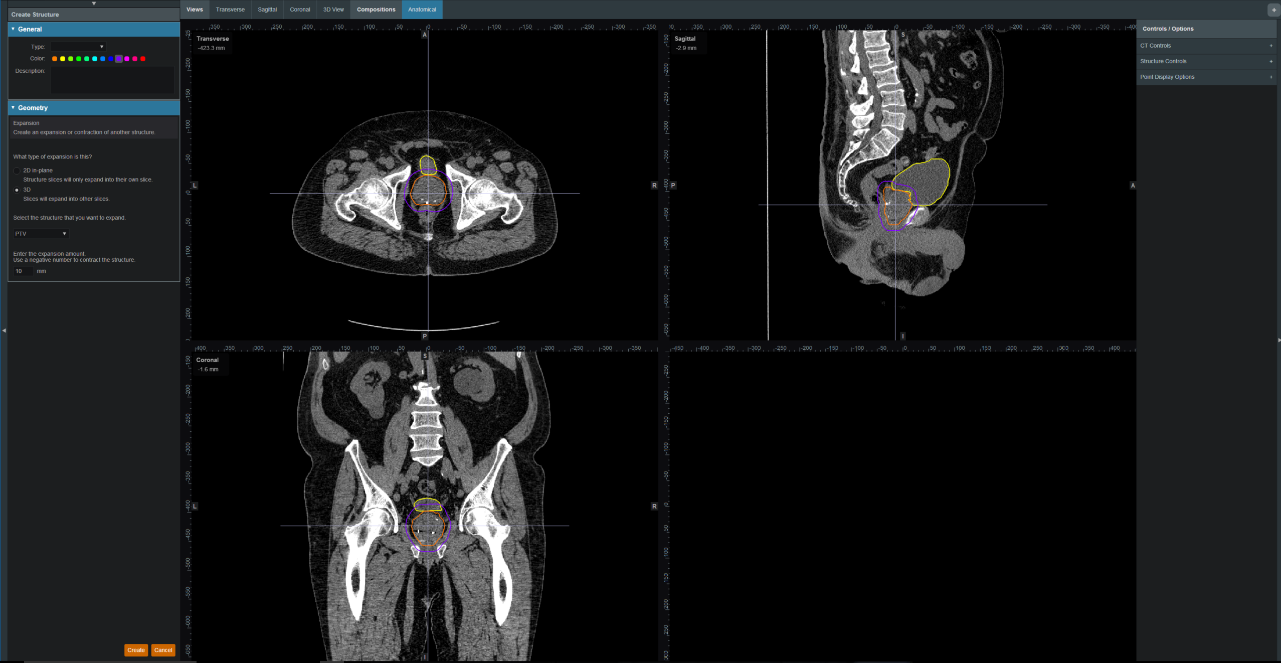
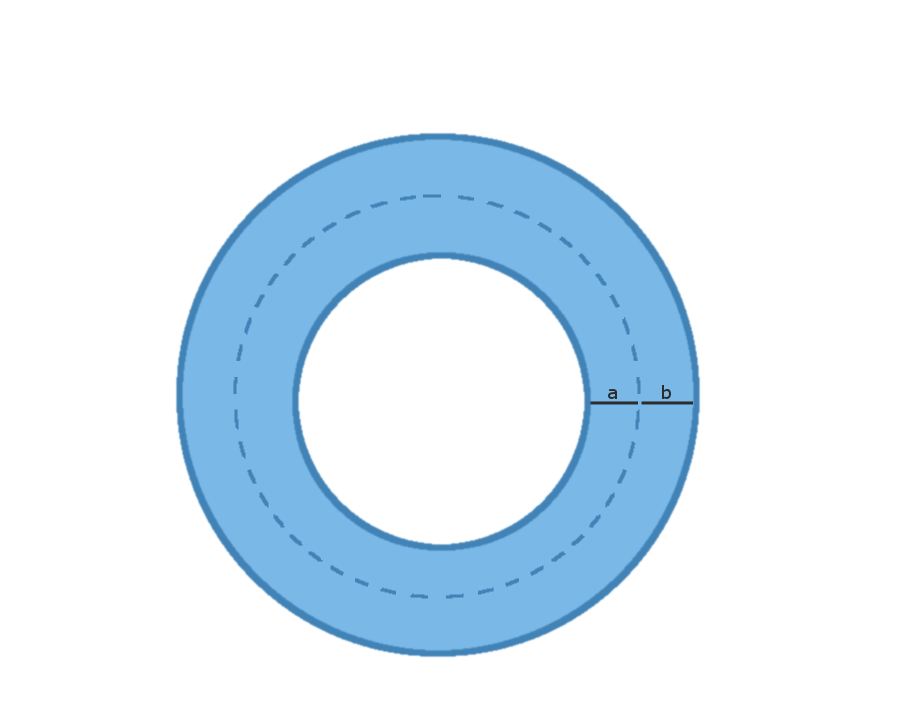
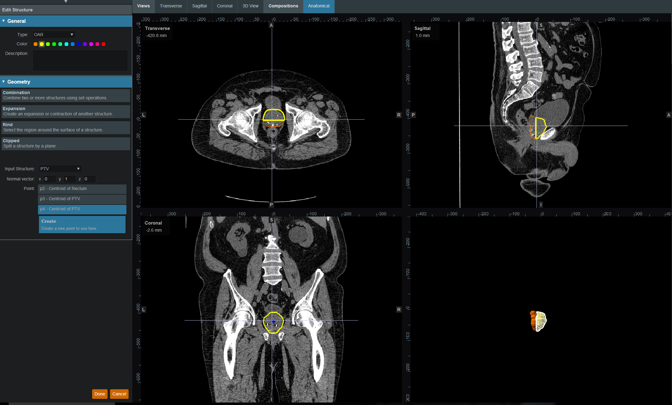